Download
1 / 22
220 likes | 415 Vues
Predictability of Seasonal Prediction. Perfect prediction. Correlation skill of Nino3.4 index. Theoretical limit (measured by perfect model correlation). Predictability gap. Actual predictability (from DEMETER). Anomaly correlation. Gap between theoretical limit & actual predictability

E N D
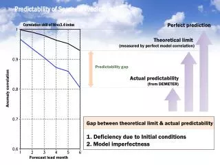
Predictability of Seasonal Prediction Perfect prediction Correlation skill of Nino3.4 index Theoretical limit (measured by perfect model correlation) Predictability gap Actual predictability (from DEMETER) Anomaly correlation Gap between theoretical limit & actual predictability 1. Deficiency due to Initial conditions 2. Model imperfectness Forecast lead month
Statistical correction (SNU AGCM) Before Bias correction After Bias Correction Predictability over equatorial region is not improved much
Is post-processing a fundamental solution? model imperfectness poor initial conditions Forecast error comes from Model improvement Good initialization process is essential to achieve to predictability limit
Issues in Climate Modeling • (Towarda new Integrated Climate Prediction System) Climate Dynamics Laboratory Seoul National University Sung-Bin Park Yoo-Geun Ham Dong min Lee Daehyun Kim Yong-Min Yang Ildae Choi Won-Woo Choi
MJO prediction ECMWF forecast (VP200, Adrian Tompkins) Analysis Forecast Lack of MJO in climate models : Barrier for MJO prediction
(a) Control Simplified Arakawa-Schubert cumulus convection scheme Relaxed Arakawa-Schubert scheme (b) Modified (b) Modified (a) Control Impact of Cumulus Parameter (a) RAS (b) McRAS Large-scale condensation scheme Influence of Cloud- Radiation Interaction Physical parameterization Problem Solution Solution Problem Loose convection criteria suppress the well developed large-scale eastward waves Unrealistic precipitation occurs over the warm but dry region Minimum entrainment constraint Relative Humidity Criterion Absence of cloud microphysics Prognostic clouds & Cloud microphysics (McRAS) Cloud-radiation interaction suppress the eastward waves Layer-cloud precipitation time scale
Basic Flow of model development Multi-Scale Prediction System Next Generation Climate Model (Global Cloud Resolving Model) Fully Coupled Model (Unified moist processes) Initialization Ocean/land/Air Air-Sea Coupling Convection Radiation Cloud Microphysics Interaction with Hydrometer Ocean (Sea ice) CRM Coupling convection and boundary layer Coupling Radiation and Aerosol Turbulence Characteristics Interaction with Hydrometer Coupling Land Surface and Ocean Surface flux & Cloud Boundary Layer Aerosol Land surface Coupling Land Surface and boundary layer Coupling Land Surface and Aearosol
Problem : cloud top sensitivity to environmental moisture Prescribed profile • Updraft mass flux Cloud resolving model (CNRM CRM) Single column model (SNUGCM) Pressure 30% 50%70% 90% Pressure 30% 50%70% 90% RH(%) * temperature and specific humidity are nudged with 1 hour time scale kg m/s kg m/s
Problem : cloud top sensitivity to environmental moisture • Single column model (Parameterization) Updraft mass flux Moistening Relative humidity 30% 50% 70% 90% 30% 50%70% 90% Pressure Pressure Pressure kg m/s kg/kg/day % Detrainment occurs at the similar level regardless of environmental moisture Cloud top is insensitive to environmental moisture Too high relative humidity produced
Effect of turbulence on convection Delayed convection relative to the turbulence initiation Cloud liquid water Turbulent kinetic energy t = +10hr t = 0hr
Delaying effect • Heat transport by turbulence • Accumulation of MSE above turbulence raising instability (t = t1) • Convection initiated (t = t2) • Convection and boundary layer turbulence coupling • Interactions between hydrometeors • Heat exchange between hydrometeors (t = t3) deep convection • Microphysical cloud model Moistening Interaction between hydrometeors Latent/ sensible heat Transport by turbulence Convection initiation time t = t0 t = t1 t = t2 t = t3
Future Plans II Cloud microphysics GCM Water vapor Precipitation f(Mass flux) Cloud water Cloud ice Validation Implementation of cloud microphysics Snow Rain Graupel CRM Prognostic equations of cloud microphysics
Future Plans II Improvement of Land Surface process Transpiration by moisture stress Heterogeneity of land data Desborough (1997) Arola and Lettenmaier(1996) * Update land surface using high resolution data Surface runoff Canopy layer River network Routing Surface layer * USGS/EROS 1km vegetation type Liston and Wood (1994) Root zone Ground runoff Soil moisture with river routing Deep soil Source for fresh water in coupled model
Works have been done: Aerosol Module Frame Aerosol module in Climate model Direct Radiation Aerosol Climate Cloud microphysics Indirect Radiation Advection Diffusion Gravity settling Wet deposition Mobilization Dry deposition
Development of Fully Coupled Model Fully Coupled Model (Unified moist processes) Unified moist processes Air-Sea Coupling Ocean (Sea ice) Cloud Microphysics Convection Radiation Coupling convection and boundary layer Coupling Radiation and Aerosol CRM Boundary Layer Aerosol Coupling Land Surface and Aearosol Land surface Coupling Land Surface and boundary layer
Development of Global Cloud Resolving Model Next Generation Model (Global Cloud Resolving Model) Air-Sea Coupling Ocean (Sea ice) Global Simulation with 20-30km (Ideal boundary condition/spherical coordinate) CRM
100km resolution Resolution dependency • 3 hourly precipitation 300km resolution 20km resolution
Description of CRM GCE-Goddard Cumulus Ensemble Cloud resolving model • Good tool for evaluation of the interaction in nature • Good substitution of observation Updraft mass flux GCE simulation The Goddard Cumulus Ensemble (GCE) model was created at 1993 by Wei-Kuo Tao. SNUAGCM single column model • Non-hydrostatic • Explicit interaction between boundary layer turbulence and convection • Sophisticated representation of microphysical processes • Physically based representation of precipitation process
Physics process of CRM Cloud and Radiation interaction Tao et al. (1996) Cloud-Top cooling Physics process of CRM Clear region cooling Clear region cooling Cloud-Base warming Stratiform Convective Turbulent kinetic energy process Tao and Simpson (1993) • Attempt to parameterization flux of prognostic quantities due to unresolved eddies (1.5 order scheme) where stability shear diffusion dissipation
Future plan: global cloud resolving model Maximize realism of model simulation Physics complexity Goal Coarse resolution test of CRM High resolution CRM On-going work Done Low resolution GCM High resolution GCM resolution Global cloud resolving model can be the best tool to simulate the nature.
GCE DYNAMICS MICROPHYSICS SURFACE FLUX RADIATION • Future plan: global cloud resolving model Global Test Dynamics and Physics of GCE Aqua-Planet simulation Test simulation of 25km resolution (1536 x 768) Non-hydrostatics dynamical core, Physics test to step by step Consider surface flux of ocean type first Hybrid approach of explicit or parameterized convection scheme Example, NICAM (Japan)