Decadal Prediction and Predictability

1. Decadal Prediction and Predictability Presenter: Edwin K. Schneider COLA SAC Meeting September 2011

2. Research Areas • Decadal prediction and predictability using the NCEP CFS (version 2) CGCM. Extension of NWP, seasonal, decadal forecasting to decadal time scales. • Understanding the mechanisms and predictability of Atlantic decadal variability, currently in a CGCM (CCSM/CESM). • Long-standing project (Schneider and Kinter 1994; discovered the AO and AAO, but didn’t comment on AO). • Issues in climate change, including role of ocean dynamics, aerosol effects, and the expansion of the tropics.

3. Major Results • Decadal prediction • We have completed CMIP5 core decadal forecasts with CFSv2/NEMOVAR, which are now being evaluated. • We are wrestling with the model bias issue and making some progress. • We are pushing beyond CMIP5, in collaboration with other groups (e.g. NCEP parallel runs, IRI, GSFC). • Mechanisms of decadal variability • We are developing a better understanding of mechanisms of interannual to decadal SST variability and the interactions between internal and externally forced variability in “perfect model” simulations. • We are settling a controversy: Do AMIP simulation have a fundamental flaw in simulating the SST forced response of the atmosphere? Answer: no. • Issues in climate change (please see Jian Lu’s poster): • Role of Wind-Evaporation-SST (WES) feedback:Wind stress “overriding” experiments with CCSM3. • WES feedback is of major importance to explain the response to doubled CO2 SST and precipitation patterns in the tropics. • WES is important for the Southern Annular mode internal variability.

4. Research Area 1Decadal Prediction • Decadal prediction and predictability using the NCEP CFS (version 2) CGCM. • COLA Team: Cash, DelSole, Huang, Kinter, Klinger, Krishnamurthy, Lu, Marx, Schneider, Stan, Zhu • Collaborations: NCEP EMC and CPC; IRI; GSFC (Thanks to NCEP for providing the model, data sets and some technical assistance)

5. Project Plan • Complete and analyze the CMIP5 “core” hindcast/forecast cases as a baseline. • Produce additional runs to address problems with the experimental design. • Conduct additional experiments to address issues of model bias, improve the hindcasts.

6. Technical Description • Model • CFS version 2 provided by NCEP EMC (identical to model used by NCEP for operational S-I prediction and CMIP5) • Initial data • Atmosphere, land, sea ice: CFSR reanalysis (1980-present) • Ocean: NEMOVAR (ECMWF) interpolated to CFS (1960-present) • 4-member ensembles • 10 year predictions from Nov. 1960, 1965, 1970, 1975, 1980, 1985, 1990, 1995, 2000, 2005 • Extend to 30 years for 1960, 1980, 2005 cases • Computer resources • NASA Pleiades (Thanks to NAS)

7. CFS v2 • An atmosphere of T126L64 • An interactive ocean with 40 levels in the vertical, to a depth of 4737 m, and horizontal resolution of 0.25 degree at the tropics, tapering to a global resolution of 0.5 degree northwards and southwards of 10N and 10S respectively • An interactive 3 layer sea-ice model • An interactive land model with 4 soil levels

8. Results: Biases • Bias, defined as forecast minus verification as a function of lead time. • Average of all lead times • Evolution high latitudes • Bias development year 1 • Verification data is NCEP/NCAR reanalysis 2m air temperature (NB: too cold in high latitudes vs. CFSRR).

9. Mean Bias T2mAveraged Years 0-10 Small bias in tropics Large bias in high latitudes

10. Bias Evolution T2m 65°N to 75°N 65°S to 75°S

11. Sea Ice/AMOC/Salinity Biases: Bohua Huang’s talk

12. Results: Ensemble Mean Hindcast Anomalies • NINO3.4 SST index • North Atlantic AMV SST index • Ensemble mean for each hindcast • Annual cycle removed

13. NINO3.4 Decadal Hindcasts

14. Obs NINO3.4 SSTA HindcastsIndividual Cases Model

15. NINO 3.4 SSTA Forecast Scores Correlation RMS Error Rebound of skill in year 2: Tim DelSole will return to this issue.

16. North Atlantic AMV Index(SST Averaged 0N-60N, 300E-360E) Observations Hindcasts

17. North Atlantic AMV Index(SST Averaged 0N-60N, 300E-360E) Observations Bias Corrected Hindcasts

18. AMV SSTA Forecast Scores Correlation RMS Error

19. Possible Issue • Initial state choice • CMIP5 protocol: Limited number of initial years may lead to biased evaluations. • Suggest that a better experimental design for the same cost might be to sample the initial states more thoroughly with fewer ensemble members.

20. Summary Decadal Prediction • Multiyear predictability of ENSO has been found. • Is this real or does it reflect inadequate sampling of initial conditions? • Have noticed some problems and have had some success in addressing biases. • Inadequate AMOC strength and variability is a serious model bias. • Decadal predictability in the North Atlantic has been identified, associated with the long term warming trend. • What is the source of this trend? • What is the source of the skill? (probably not AMOC)

21. Research Area 2:Mechanisms of Decadal Variability • Understanding the mechanisms and predictability of Atlantic decadal variability in a CGCM (CCSM/CESM). • Research group • COLA/GMU: Schneider, Huang, Chen, Colfescu • Collaboration: RSMAS – Kirtman group

22. Motivation • Diagnose and understand the mechanisms of simulated low frequency Atlantic SST variability. • In particular, what were the roles of weather noise forcing, coupled feedbacks, and ocean dynamics? • What are the implications for “decadal” predictability?

23. Approach • Perfect model/perfect data framework • Isolate the weather noise in a CGCM simulation. • Force an Interactive Ensemble CGCM (IE-CGCM) with the weather noise in controlled experiments.

24. Data and Models • NCAR CCSM • CCSM3 (T85 x 1 and T42 x 1) • 300 year control simulation (T42 x 1) • 20C3M 1980-2000 simulation (T85 x 1) • CAM3 (AGCM component of CCSM3) + CLM3 (LSM component of CCSM3) • Interactive ensemble CCSM3 • Ensemble mean of 6 copies of CAM3 coupled to ocean, land, sea ice • T42 x 1

25. NCAR CCSM3 • Is an appropriate model for this study. • It produces reasonable simulations of decadal/multidecadal modes of SST variability (i.e., you might guess that this was a model of Earth). • NAO, AMV, TAV

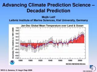
26. Atlantic Multidecadal Variability “Obs” (130 years) “Ctrl” (300 years) 0.5 0.5 0 0 -0.5 -0.5 1880 1900 1920 1940 1960 1980 2000 720 750 780 810 840 870 900 930 960 990 Fig.5 Upper panel: regression of SST anomalies against its normalized AMV index. Lower panel: AMV index. The red curves are the annual mean and the black curves indicate the 11-year running mean with high frequency removed. Data are detrended.

27. Weather Noise Forced Interactive Ensemble … Response 1 Response 2 Response N … AGCM AGCM AGCM 1 2 N Ensemble Mean Surface Fluxes SST Weather Noise Surface Fluxes OGCM

28. Response to Observed External Forcing CCSM3 and IE-CCSM3 1870-2000 (20C3M) CCSM3 CMIP4 Global Means Ts Z 500 15 .4 -.4 Red = CCSM3 ensemble mean Blue = CCSM3 IE -15 1870 1980 1870 1980 .04 Precip Ts .4 Colors= ensemble members Black= ensemble mean -.4 -.04

29. Experimental Design Weather Noise Total (from “Ctrl”) “Signal”

30. Controversy!Important for Our Method! • No SST forced AGCM produces a realistic response to observed SST. • Is this due to fundamental flaw in uncoupled vs. coupled simulations? • This is the result described in publications: Wu and Kirtman (2004), Wang et al. (2005). • Is this due to model bias? • Test in a perfect model framework to eliminate model bias (see Hua Chen’s poster-includes comparison with results from above papers).

31. Answer!Important for Our Method! • No SST forced AGCM produces a realistic response to observed SST. • Is this due to fundamental flaw in uncoupled vs. coupled simulations? No • Is this due to model bias?

32. Answer!Important for Our Method! • No SST forced AGCM produces a realistic response to observed SST. • Is this due to fundamental flaw in uncoupled vs. coupled simulations? No • Is this due to model bias? Yes: there is no other possibility.

33. Linear Trends in the Tropics 4. Copsey, D., R. Sutton, and J. R. Knight, 2006: Recent trends in sea level pressure in the Indian Ocean region. GRL, 33.

34. Trends 1950-1996 Copsey et al. CCSM3 20C3M SST SLP Obs CGCM SLP AGCM

35. On the Limitations of Prescribing Sea Surface Temperatures in Atmospheric General Circulation Model Experiments James W. Hurrell1*, Simon Brown2, Adam Phillips1, and Christophe Cassou1 1National Center for Atmospheric Research, Boulder, CO, USA. 2United Kingdom Meteorological Office, Bracknell, U.K. *Corresponding author email: jhurrell@ucar.edu Climate Dynamics April 2004 (unpublished, figures lost)

36. Hurrell et al’s Comparison • Examined ratio of standard deviations CGCM:AGCM. • Their results appear to agree with predictions of Barsugli and Battisti (1998) model. • Our results appear to agree with Hurrell et al’s., and additionally provide support to Barsugli and Battisti’s assumptions. • Our determination of weather noise is in fact based on Hurrell et al’s “limitations.”

37. Point Correlation of SST IE-CCSM3 with Global Noise Forcingvs.CCSM3 Control (“Truth”) Monthly Anomalies Annual Anomalies => Most of the SST variability is weather noise forced.

38. IE Experiments Global weather noise Weather noise in Whole Atlantic only …

39. Summary Decadal Prediction • Our decadal prediction project is well under way, using CFS_v2, and is generating questions: • ENSO skill rebound? • Sampling of initial states? • Biases North Atlantic and polar regions? • Source of skill in hindcasting AMV?

40. Summary - Decadal Mechanisms • Contrary to some findings in the literature, we find (in CCSM3) that AMIP simulations are able to capture the SST-forced response of the atmosphere. • Weather noise and external forcing are the major sources of SST variability in CCSM3. • Weather noise is the cause of variability about the ensemble mean for the CCSM3 20C3M ensemble. • Using our method, we will arrive at a reasonably complete understanding of the mechanisms of decadal variability in CGCMs.