Download
1 / 31
310 likes | 486 Vues
Empirical Models of SEASONAL to decadal variability and predictability . Matt Newman and Mike Alexander CIRES/University of Colorado and NOAA/ESRL/PSD. 2010-2060 “A1B” tropical trends, same model, different ensemble members. Outline of Talk.

E N D
Empirical Models of SEASONAL to decadal variability and predictability Matt Newman and Mike Alexander CIRES/University of Colorado and NOAA/ESRL/PSD
2010-2060 “A1B” tropical trends, same model, different ensemble members
Outline of Talk • Multivariate red noise: a basic model of Pacific climate variability • Applied to: • Tropics • Pacific Basin (PDO) • Decadal forecasts of global surface temperature anomalies
Some requirements for empirical climate models • Capture the evolution of anomalies • Growth/decay, propagation • need anomaly tendency: dynamical model • Can relate to physics/processes and estimate predictability? • Limited data + Occam’s razor = not too complex • How many model parameters are enough? • Problem: is model fitting signal or noise? • Test on independent data (or at least cross-validate) • Testable • Is the underlying model justifiable? • Where does it fail? • Can we understand where/why it succeeds? (no black boxes) • Previous success of linear diagnosis/theory for climate suggest potential usefulness of linear empirical dynamical model
For example, surface heat fluxes due to rapidly varying weather driving the ocean might be approximated as Two types of linear approximations • “Linearization” : amplitude of nonlinear term is small compared to amplitude of linear term • Then ignore nonlinear term • “Coarse-grained” : time scale of nonlinear term is small compared to time scale of linear term • Then parameterize nonlinear term as (second) linear term + unpredictable white noise: N(x) ~ Tx + ξ
“Multivariate Red Noise” null hypothesis • Noise/response is local (or an index) • For example, air temperature anomalies force SST • use univariate (“local”) red noise: dx/dt = bx + fswhere x(t) is a scalar time series, b<0, and fs is white noise • Noise/response is non-local: patterns matter • For example, SST sensitive to atmospheric gradient • use multivariate (“patterns-based”) red noise: dx/dt = Bx + Fswhere x(t) is a series of maps, B is stable, and Fs is white noise (maps) • Note that B is a matrix and x and Fs are vectors • If B is not symmetric* (*nonnormal), transient anomaly growth is possible even though exponential growth is not • How can we determine B?
Linear inverse model (LIM) “Inverse method”– derive B from observed statistics If the climate state x evolves as dx/dt = Bx+ FS then τ0-lagand zero-lag covariance are related as C(τ0) = G(τ0) C(0) = exp(Bτ0) C(0) [where C(τ) = <x(t+τ)x(t)T>]. • LIM procedure: • Prefilter data in EOF space (since B = logm [C(τ0)C(0)-1]/τ0) • Determine B from one training lag τ0. • Test for linearity • For much longer lagsτ, is C(τ) = exp(Bτ) C(0) ? • This “τ-test”is key to LIM. • Cross validate hindcasts (withhold 10% of data)
Linear inverse model (LIM), cont. “Inverse method”– derive B from observed statistics If the climate state x evolves as dx/dt = Bx+ FS then ensemble mean forecast at leadτis x(τ) = exp(Bτ) x(0) . Eigenmodes of Bare all damped but can be either stationary or propagating*(*Bei = λiei , where λi can be complex) & not orthogonal. When Bis “nonnormal” (dynamics are not symmetric) transient “optimal” anomaly growth can occur*(*DG(τ)vi= σiui, where D is a norm), leading to greater predictability.
ENSO flavors Newman, M., S.-I. Shin, and M. A. Alexander, 2011: Natural variation in ENSO flavors. Geophys. Res. Lett., L14705, doi:10.1029/2011GL047658.
“Multivariate Red Noise” null hypothesis dx/dt = Bx + Fswhere x(t) is a series of maps, B is stable, and Fs is white noise (maps) • Determine Band Fsusing “Linear Inverse Model” (LIM) • x is SST/20 C depth/surface zonal wind stress seasonal anomalies in Tropics, 1959-2000 (Newman et al. 2011, Climate Dynamics) • prefiltered in reduced EOF space (23 dof) • LIM determined from specified lag (3 months) as in AR1 model • Extension of work by Penland and co-authors (e.g. Penland and Sardeshmukh 1995)
Verifying Multivariate Red Noise: compare observed and LIM-predicted lag-covariances and spectra Note that LIM entirely determined from one-season lag statistics
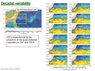
Multivariate red noise captures “optimal” evolution of ENSO types SST: shading Thermocline depth: contours Zonal wind stress: arrows
Optimal structures are relevant to observed EP and CP ENSO events Composite: Six months after a > ± 1 sigma projection (blue dots) on either the first or second optimal initial condition, constructed separately for warm and cold events Green dots represent mixed EP-CP events
Multidecadal variations of CP/EP ENSOs driven by noise “Increasing CP/EP Cases” : Adjacent 60-yr segments where CP/EP ratio increases r(Nino3,Nino4) decreases 24000 yr LIM “model run”: dx/dt = Bx + Fs Values determined over 30-yr intervals spaced 10 years apart
LIM can provide realistic synthetic dataNino 3.4 times series: DJF (gray) and 25-yr running mean (black)Multi-proxy reconstruction (Emile-Geay 2012), one of 100 LIM realizations, forced CCSM4 show decadal signal, CCSM4 control does not
pacific sst empirical models Newman, M., 2007: Interannual to decadal predictability of tropical and North Pacific sea surface temperatures. J. Climate, 20, 2333-2356. Alexander, M. A., L. Matrosova, C. Penland, J. D. Scott, and P. Chang, 2008: Forecasting Pacific SSTs: Linear Inverse Model Predictions of the PDO. J. Climate, 21, 385-402. Newman, M., D. Smirnov, and M. Alexander, 2012: Relative impacts of tropical forcing and extratropical air-sea coupling on air/sea surface temperature variability in the North Pacific. In preparation.
PDO depends on ENSO (Newman et al. 2003) Forecast: PDO (this year) = .6PDO(last year) + .6ENSO(this year) “reddened ENSO” r=.74
“Multivariate Red Noise” null hypothesis dx/dt = Bx + Fswhere x(t) is a series of maps, B is stable, and Fs is white noise (maps) • Determine Band Fsusing “Linear Inverse Model” (LIM) • x is SST seasonal anomalies in the Pacific (30°S-60°N), 1950-2000 (Alexander et al. 2008, J. Climate) • prefiltered in reduced EOF space (13 dof) • LIM determined from specified lag (3 months) as in AR1 model • Skill in predicting Nino3.4 and PDO > 0.6 for 1 year forecasts when initialized in late winter
Diagnosing coupling • Use slightly different LIM by separating Tropics and North Pacific: • Define xtropics =SST/20 C depth/surface zonal wind stress TNorthPac=SST (20ºN-60ºN) • Coupling effects are determined by zeroing out the appropriate submatrices within B.
Diagnosing coupling • Use slightly different LIM by splitting Tropics and North Pacific: • Define xtropics =SST/20 C depth/surface zonal wind stress TNorthPac=SST (20ºN-60ºN) • Coupling effects are determined by zeroing out the appropriate submatrices within B. Decouple Tropics from North Pacific, then recalculate statistics given same noise
Impact of tropical coupling on SST variability Variance 6 month lag covariance LIM Uncoupled East Pacific SST variability almost entirely due to tropical forcing. In WBC, most variability is independent of the Tropics.
Dominant “internal” North Pacific SST mode Compute new EOFs from covariance matrix determined from uncoupled LIM
“Multivariate Red Noise” null hypothesis dx/dt = Bx + Fswhere x(t) is a series of maps, B is stable, and Fs is white noise (maps) • Determine Band Fsusing “Linear Inverse Model” (LIM) • x is SST annual mean (July-June) anomalies in Tropics and North Pacific, 1900-2001 (Newman 2007) • prefiltered in reduced EOF space (10dof) • LIM determined from specified lag (1 year) as in AR1 model
Components of the PDO Leading eigenmodesof B, with time series (1900-2001) • Eigenmodes represent: • Trend • “Pacific Multidecadal Oscillation” (PMO) • “Decadal ENSO” • Almost all long range skill contained in first 2 eigenmodes
“Regime shifts” “PMO” Constructing the PDO from a sum of three red noise processesTime series show projection of each mode onto the PDO “Decadal ENSO” “Interannual ENSO” Reconstructed PDO PDO = PMO +Decadal ENSO +Interannual ENSO PDO
Decadal forecasts of global surface temperature Newman, M., 2012: An empirical benchmark for decadal forecasts of global surface temperature anomalies. J. Climate, in review (minor revision).
Multivariate red noise surface temperatures dx/dt = Bx + Fs • Determine Band Fsusing “Linear Inverse Model” (LIM) • x is SST/Land (2m) temperature, 12-month running mean anomalies, 1900-2008 (Newman 2012) • prefiltered in reduced EOF space (20 dof) • LIM determined from specified lag (12 months) as in AR1 model
Years 2-5 Years 6-9 Decadal skill for forecasts initialized 1960-2000LIM has clearly higher skill than damped persistence, comparable skill to CMIP5 CGCM decadal “hindcasts” LIM
Leading eigenmodesof B, with time series (1900-2008) Eigenmodes represent: Trend Atlantic Multidecadal Oscillation (AMO) Pacific Multidecadal Oscillation (PMO) Almost all skill contained in these 3 eigenmodes Enhanced LIM PDO skill due to PMO
Conclusions • North Pacific Climate Variability • Sum of “reddened” ENSO + northwest Pacific-based (KOE?) variability • Coupled GCMs may underpredict the second process • LIM is a good model of climate • Captures statistics of anomaly evolution and makes forecasts • Serves as a benchmark for numerical models • Can diagnose dynamical relationships between different variables/locations and how they provide/limit predictability • Can generate long runs of realistic synthetic “data” • Consistent with apparent “regime shifts” with limited predictability • Uses of climate variability • for scenario building to test sensitivity of ecosystem • to make predictions of ecosystem