Comprehensive Overview of CPU Scheduling: Concepts, Algorithms, and Performance Criteria
This document provides an in-depth look at CPU scheduling, covering basic concepts and various algorithms used in managing CPU resources. Key topics include scheduling criteria like CPU utilization, throughput, turnaround time, and response time. It explores both preemptive and non-preemptive scheduling methods such as First-Come, First-Served (FCFS), Shortest Job First (SJF), and Round Robin (RR). Additionally, it discusses the impact of multiprogramming on CPU efficiency and provides examples for better understanding the scheduling decisions made within operating systems like BSD UNIX.


Comprehensive Overview of CPU Scheduling: Concepts, Algorithms, and Performance Criteria
E N D
Presentation Transcript
CPU Scheduling • Basic Concepts • Scheduling Criteria • Scheduling Algorithms • Scheduling in BSD UNIX
Basic Concepts • Maximum CPU utilization obtained with multiprogramming • CPU–I/O Burst Cycle – Process execution consists of a cycle of CPU execution and I/O wait. • CPU burst distribution
CPU Scheduler • Selects from the Ready processes in memory • CPU scheduling decisions occur when process: 1. Switches from running to waiting state. 2. Switches from running to ready state. 3. Switches from waiting to ready. 4. Terminates. • Scheduling under 1 and 4 is nonpreemptive. • All other scheduling is preemptive.
Dispatcher • Dispatcher module gives control of the CPU to the process selected by the short-term scheduler; this involves: • switching context • switching to user mode • jumping to the proper location in the user program to restart that program • Dispatch latency– time it takes for the dispatcher to stop one process and start another running.
Scheduling Criteria • CPU utilization – Percent time CPU busy • Throughput – # of processes that complete their execution per time unit • Turnaround time –time to execute a process: from start to completion. • Waiting time –time in Ready queue • Response time – amount of time it takes from when a request was submitted until the first response is produced, not output (for time-sharing environment)
Optimization Criteria • Max CPU utilization • Max throughput • Min turnaround time • Min waiting time • Min response time
P1 P2 P3 0 24 27 30 First-Come, First-Served (FCFS) • Example: ProcessBurst Time P1 24 P2 3 P33 • Assume processes arrive as: P1 , P2 , P3 The Gantt Chart for the schedule is: • Waiting time forP1 = 0; P2= 24; P3= 27 • Average waiting time: (0 + 24 + 27)/3 = 17
P2 P3 P1 0 3 6 30 FCFS Scheduling (Cont.) Suppose processes arrive as: P2 , P3 , P1 . • The Gantt chart for the schedule is: • Waiting time for P1 = 6;P2 = 0; P3 = 3 • Average waiting time: (6 + 0 + 3)/3 = 3 • Much better than previous case. • Convoy effector head-of-line blocking • short process behind long process
Shortest-Job-First (SJR) Scheduling • Process declares its CPU burst length • Two schemes: • non-preemptive – once CPU assigned, process not preempted until its CPU burst completes. • Preemptive – if a new process with CPU burst less than remaining time of current, preempt. Shortest-Remaining-Time-First (SRTF). • SJF is optimal – gives minimum average waiting time for a given set of processes.
P1 P3 P2 P4 0 3 7 8 12 16 Example of Non-Preemptive SJF Process Arrival Time Burst Time P1 0.0 7 P2 2.0 4 P3 4.0 1 P4 5.0 4 • SJF (non-preemptive) • Average waiting time • = (0 + 6 + 3 + 7)/4 - 4
P1 P2 P3 P2 P4 P1 11 16 0 2 4 5 7 Example of Preemptive SJF ProcessArrival TimeBurst Time P1 0.0 7 P2 2.0 4 P3 4.0 1 P4 5.0 4 • SJF (preemptive) • Average waiting time • = (9 + 1 + 0 +2)/4 - 3
Determining Next CPU Burst • Can only estimate the length. • Can be done by using the length of previous CPU bursts, using exponential averaging.
Examples of Exponential Averaging • =0 • n+1 = n • Recent history does not count. • =1 • n+1 = tn • Only the actual last CPU burst counts. • If we expand the formula, we get: n+1 = tn+(1 - ) tn -1 + … +(1 - ) j tn -1 + … +(1 - ) n=1 tn 0 • and (1 - ) are <= 1, so each successive term has less weight than its predecessor.
Priority Scheduling • Priority associated with each process • CPU allocated to process with highest priority • Preemptive or non-preemptive • Example - SJF: priority scheduling where priority is predicted next CPU burst time. • Problem: Starvation • low priority processes may never execute. • Solution: Aging • as time progresses increase the priority of the process.
Round Robin (RR) • Each process assigned a time quantum, usually 10-100 milliseconds. After this process moved to end of the Ready Q • n processes in ready queue, time quantum = q, then each process gets 1/n of the CPU time in chunks of at most q time units at once. No process waits more than (n-1)q time units. • Performance • q large FIFO • q small q must be large with respect to context switch, otherwise overhead too high.
P1 P2 P3 P4 P1 P3 P4 P1 P3 P3 0 20 37 57 77 97 117 121 134 154 162 Example: RR, Quantum = 20 ProcessBurst Time P1 53 P2 17 P3 68 P4 24 • The Gantt chart is: • Typically, higher average turnaround than SJF, but better response.
Small Quantum Increased Context Switches
Multilevel Queue • Ready queue partitioned into separate queues: • foreground (interactive) and background (batch) • Each queue has its own scheduling algorithm, foreground – RR, background – FCFS • Scheduling between queues. • Fixed priority scheduling; Possible starvation. • Time slice: i.e., 80% to foreground in RR, 20% to background in FCFS
Multilevel Feedback Queue • A process can move between the various queues; aging can be implemented this way. • Multilevel-feedback-queue scheduler defined by: • number of queues • scheduling algorithms for each queue • method used to select when upgrade process • method used to select when demote process • method used to determine which queue a process will enter when that process needs service
Example: Multilevel Feedback Queue • Three queues: • Q0 – time quantum 8 milliseconds • Q1 – time quantum 16 milliseconds • Q2 – FCFS • Scheduling • A new job enters queue Q0served by FCFS. Then job receives 8 milliseconds. If not finished in 8 milliseconds, moved to Q1. • At Q1 job served by FCFS. Then receives 16 milliseconds. If not complete, preempted and moved to Q2.