Technology and Cost
280 likes | 401 Vues
Understand the neoclassical view of firms, cost analysis, economies of scale, and market structure. Learn how firms minimize costs and make output decisions to maximize profit. Explore ray average cost for multi-product firms.

Technology and Cost
E N D
Presentation Transcript
Technology and Cost Chapter 4: Technology and Cost
The Neoclassical View of the Firm • Concentrate upon a neoclassical view of the firm • the firm transforms inputs into outputs Inputs Outputs The Firm • There is an alternative approach (Coase) • What happens inside firms? • How are firms structured? What determines size? • How are individuals organized/motivated? Chapter 4: Technology and Cost
The Single-Product Firm • Profit-maximizing firm must solve a related problem • minimize the cost of producing a given level of output • combines two features of the firm • production function: how inputs are transformed into output Assume that there are n inputs at levels x1 for the first, x2 for the second,…, xn for the nth. The production function, assuming a single output, is written: q = f(x1, x2, x3,…,xn) • cost function: relationship between output choice and production costs. Derived by finding input combination that minimizes cost n wixi Minimize subject to f(x1, x2, x3,…,xn) = q1 xi i=1 Chapter 4: Technology and Cost
This analysis has interesting implications • different input mix across • time: as capital becomes relatively cheaper • space: difference in factor costs across countries • Analysis gives formal definition of the cost function • denoted C(Q): total cost of producing output Q • average cost = AC(Q) = C(Q)/Q • marginal cost: • additional cost of producing one more unit of output. • Slope of the total cost function • formally: MC(Q) = dC(Q)/d(Q) • Also consider sunk cost • incurred on entry independent of output • cannot be recovered on exit Chapter 4: Technology and Cost
Cost curves: an illustration Typical average and marginal cost curves $/unit Relationship between AC and MC MC If MC < AC then AC is falling AC If MC > AC then AC is rising MC = AC at the minimum of the AC curve Quantity Chapter 4: Technology and Cost
Cost and Output Decisions • Firms maximizes profit where MR = MC provided • output should be greater than zero • implies that price is greater than average variable cost • shut-down decision • Enter if price is greater than average total cost • must expect to cover sunk costs of entry Chapter 4: Technology and Cost
Economies of scale • Definition: average costs fall with an increase in output • Represented by the scale economy index AC(Q) S = MC(Q) • S > 1: economies of scale • S < 1: diseconomies of scale • S is the inverse of the elasticity of cost with respect to output dC(Q) dQ dC(Q) C(Q) MC(Q) 1 hC = = = = C(Q) Q dQ Q AC(Q) S Chapter 4: Technology and Cost
Economies of scale • Sources of economies of scale • “the 60% rule”: capacity related to volume while cost is related to surface area • product specialization and the division of labor • “economies of mass reserves”: economize on inventory, maintenance, repair • indivisibilities Chapter 4: Technology and Cost
Indivisibilities, sunk costs and entry • Indivisibilities make scale of entry an important strategic decision: • enter large with large-scale indivisibilities: heavy overhead • enter small with smaller-scale cheaper equipment: low overhead • Some indivisible inputs can be redeployed • aircraft • Other indivisibilities are highly specialized with little value in other uses • market research expenditures • rail track between two destinations • The latter are sunk costs: nonrecoverable if production stops • Sunk costs affect market structure by affecting entry Chapter 4: Technology and Cost
Sunk Costs and Market Structure • The greater are sunk costs the more concentrated is market structure • An example: Lerner Index is inversely related to the number of firms Suppose that elasticity of demand h = 1 Then total expenditure E = P.Q If firms are identical then Q = Nqi Suppose that LI = (P – c)/P = A/Na Suppose firms operate in only on period: then (P – c)qi = K As a result: Chapter 4: Technology and Cost
Multi-Product Firms • Many firms make multiple products • Ford, General Motors, 3M etc. • What do we mean by costs and output in these cases? • How do we define average costs for these firms? • total cost for a two-product firm is C(Q1, Q2) • marginal cost for product 1 is MC1 = C(Q1,Q2)/Q1 • but average cost cannot be defined fully generally • need a more restricted definition: ray average cost Chapter 4: Technology and Cost
Ray average cost • Assume that a firm makes two products, 1 and 2 with the quantities Q1 and Q2 produced in a constant ratio of 2:1. • Then total output Q can be defined implicitly from the equations Q1 = 2Q/3 and Q2 = Q/3 • More generally: assume that the two products are produced in the ratio 1/2 (with 1 + 2 = 1). • Then total output is defined implicitly from the equations Q1 = 1Q and Q2 = 2Q • Ray average cost is then defined as: C(1Q, 2Q) RAC(Q) = Q Chapter 4: Technology and Cost
An example of ray average costs • Assume that the cost function is: • Marginal costs for each product are: C(Q1, Q2) = 10 + 25Q1 + 30Q2 - 3Q1Q2/2 3Q2 C(Q1,Q2) MC1 = = 25 - 2 Q1 3Q1 C(Q1,Q2) MC2 = = 30 - 2 Q2 Chapter 4: Technology and Cost
C(Q1, Q2) = 10 + 25Q1 + 30Q2 - 3Q1Q2/2 • Ray average costs: assume 1 = 2 = 0.5 Q1 = 0.5Q; Q2 = 0.5Q C(0.5Q, 0.5Q) RAC(Q) = Q 10 + 25Q/2+ 30Q/2 - 3Q2/8 10 55 3Q - + = = Q 2 8 Q Now assume 1 = 0.75; 2 = 0.25 C(0.75Q, 0.25Q) RAC(Q) = Q 10 + 75Q/4+ 30Q/4 - 9Q2/32 10 105 9Q - + = = Q 4 32 Q Chapter 4: Technology and Cost
Economies of scale and multiple products • Definition of economies of scale with a single product C(Q) AC(Q) S = = MC(Q) Q.MC(Q) • Definition of economies of scale with multiple products C(Q1,Q2,…,Qn) S = MC1Q1 + MC2Q2 + … + MCnQn • This is by analogy to the single product case • relies on the implicit assumption that output proportions are fixed • so we are looking at ray average costs in using this definition Chapter 4: Technology and Cost
The example once again C(Q1, Q2) = 10 + 25Q1 + 30Q2 - 3Q1Q2/2 MC1 = 25 - 3Q2/2 ; MC2 = 30 - 3Q1/2 Substitute into the definition of S: C(Q1,Q2,…,Qn) S = MC1Q1 + MC2Q2 + … + MCnQn 10 + 25Q1 + 30Q2 - 3Q1Q2/2 = 25Q1 - 3Q1Q2/2 + 30Q2 - 3Q1Q2/2 It should be obvious in this case that S > 1 This cost function exhibits global economies of scale Chapter 4: Technology and Cost
Economies of Scope • Formal definition C(Q1, 0) + C(0 ,Q2) - C(Q1, Q2) SC = C(Q1, Q2) • The critical value in this case is SC = 0 • SC < 0 : no economies of scope; SC > 0 : economies of scope. • Take the example: 10 + 25Q1 + 10 + 30Q2 - (10 + 25Q1 + 30Q2 - 3Q1Q2/2) > 0 SC = 10 + 25Q1 + 30Q2 - 3Q1Q2/2 Chapter 4: Technology and Cost
Economies of Scope (cont.) • Sources of economies of scope • shared inputs • same equipment for various products • shared advertising creating a brand name • marketing and R&D expenditures that are generic • cost complementarities • producing one good reduces the cost of producing another • oil and natural gas • oil and benzene • computer software and computer support • retailing and product promotion Chapter 4: Technology and Cost
Flexible Manufacturing • Extreme version of economies of scope • Changing the face of manufacturing • “Production units capable of producing a range of discrete products with a minimum of manual intervention” • Benetton • Custom Shoe • Levi’s • Mitsubishi • Production units can be switched easily with little if any cost penalty • requires close contact between design and manufacturing Chapter 4: Technology and Cost
Flexible Manufacturing (cont.) • Take a simple model based on a spatial analogue. • There is some characteristic that distinguishes different varieties of a product • sweetness or sugar content • color • texture • This can be measured and represented as a line • Individual products can be located on this line in terms of the quantity of the characteristic that they possess • One product is chosen by the firm as its base product • All other products are variants on the base product Chapter 4: Technology and Cost
Flexible Manufacturing (cont.) • An illustration: soft drinks that vary in sugar content (Diet) (LX) (Super) 0 0.5 1 Low High Each product is located on the line in terms of the amount of the characteristic it has This is the characteristics line Chapter 4: Technology and Cost
The example (cont.) (Diet) (LX) (Super) • Assume that the process is centered on LX as base product. 0 0.5 1 Low High A switching cost s is incurred in changing the process to either of the other products. There are additional marginal costs of making Diet or Super - from adding or removing sugar. These are r per unit of “distance” between LX and the other product. There are shared costs F: design, packaging, equipment. Chapter 4: Technology and Cost
The example (cont.) • In the absence of shared costs there would be specialized firms. • Shared costs introduce economies of scope. m S Total costs are: C(zj, qj) = F + (m - 1)s + [(c + rzj - z1)qj] j=1 If production is 100 units of each product: one product per firm with three firms C3 = 3F + 300c one firm with all three products C1 = F + 2s + 300c + 100r C1 < C3 if 2s + 100r < 2F F > 50r + s This implies a constraint on set-up costs, switching costs and marginal costs for multi-product production to be preferred. Chapter 4: Technology and Cost
Determinants of Market Structure • Economies of scale and scope affect market structure but cannot be looked at in isolation. • They must be considered relative to market size. • Should see concentration decline as market size increases • Entry to the medical profession is going to be more extensive in Chicago than in Oxford, Miss • Find more extensive range of financial service companies in Wall Street, New York than in Frankfurt Chapter 4: Technology and Cost 2-37
Network Externalities • Market structure is also affected by the presence of network externalities • willingness to pay by a consumer increases as the number of current consumers increase • telephones, fax, Internet, Windows software • utility from consumption increases when there are more current consumers • These markets are likely to contain a small number of firms • even if there are limited economies of scale and scope Chapter 4: Technology and Cost
The Role of Policy • Government can directly affect market structure • by limiting entry • taxi medallions in Boston and New York • airline regulation • through the patent system • by protecting competition e.g. through the Robinson-Patman Act Chapter 4: Technology and Cost
Illustration of ray average costs Chapter 4: Technology and Cost