1st Level Analysis
1st Level Analysis. Design Matrix , Contrasts & Inference. Methods for dummies 2011-12, Hikaru Tsujimura and Hsuan -Chen Wu. Design matrix. fMRI time-series. kernel. Motion correction. Smoothing. General Linear Model. Spatial normalisation. Standard template.

1st Level Analysis
E N D
Presentation Transcript
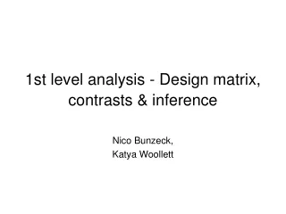
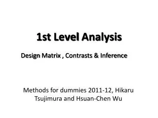
1st LevelAnalysis Design Matrix, Contrasts & Inference Methods for dummies 2011-12, HikaruTsujimura and Hsuan-Chen Wu
Design matrix fMRI time-series kernel Motion correction Smoothing General Linear Model Spatial normalisation Standard template So far, we learned preprocessing, then what is next? After realigning, filtering, spatial normalization, images are ready to be analyzed!
Outline • What is First Level Analysis? • Role of Design Matrix in analysis • Role of Contrastin analysis • How to Infer?
First level Analysis = Within Subjects Analysis Time Time Time Time Run 1 Run 1 Run 2 Run 2 First level Subject 1 Subject n Second level group(s)
Key in 1st Level Analysis The GLM for fMRI: β ε + Y X x = BOLD signal Design Matrix (Variables that explain the observed data (EV)) Relative Contributionof X to the overalldata (These need tobe estimated) Error (The difference between the observed data and that which is predicted by the model)
X = Design Matrix Time (n) Regressors(m)
Regressors – represent hypothesised contributors in your experiment. They are represented by columns in the design matrix (1column = 1 regressor) • Regressors of Interest or Experimental Regressors– represent those variables which you intentionally manipulated. The type of variable used affects how it will be represented in the design matrix • Regressors of no interest or nuisance regressors – represent those variables which you did not manipulate but you suspect may have an effect. By including nuisance regressors in your design matrix you decrease the amount of error. • E.g. -The 6 movement regressors (rotations x3 & translations x3 ) or physiological factors e.g. heart rate
Designs Block design Event- related design Intentionally design events of interest into blocks Retrospectively look at when the events of interest occurred. Need to code the onset time for each regressor
Regressors • A dark-light colour map is used to show the value of each regressor within a specific time point • Black = 0 and illustrates when the regressor is at its smallest value • White = 1 and illustrates when the regressor is at its largest value • Grey represents intermediate values • The representation of each regressor column depends upon the type of variable specified Time (n) Regressors (m)
Modelling Haemodynamics Changes in the bold activation associated with the presentation of a stimulus • Haemodynamic response function • Peak of intensity after stimulus onset, followed by a return to baseline then an undershoot • Box-car model is combined with the HRF to create a convolved regressor which matches the rise and fall in BOLD signal (greyscale) • Even with this, not always a perfect fit so can include temporal derivatives (shift the signal slightly) or dispersion derivatives (change width of the HRF response) *more later in this course HRF Convolved
Covariates • What if you variable can’t be described using conditions? • E.g Movement regressors – not simply just one state or another The value can take any place along the X,Y,Z continuum for both rotations and translations • Covariates – Regressors that can take any of a continuous range of values (parametric) • Thus the type of variable affects the design matrix – the type of design is also important
Finding the best fitting model: These optimal fitting values are saved in beta image files for each EV. The residual signal variance in the voxel, unexplained by the model (within subject error) is saved in MSres image files.
Outline • Why do we need contrasts? • What are contrasts? • T contrasts • F contrasts • Factorial design
Why do we need contrasts? • Because fMRI provides no information about absolute levels of activation, only about changes in activation over time • Research hypotheses involve comparison of activation between conditions • Researcher constructs a design matrix consisting of a set of regressors, and then determines how strongly each of those regressors matches changes in the measured BOLD signal • Regressors explain much of the BOLD signal have high magnitude parameter weights (larger β values), whereas regressors explain little of BOLD signal have parameter weights near zero Y = Xxβ+ε Matrix of BOLD signals (What you collect) Design matrix (This is what is put into SPM) Matrix parameters (These need to be estimated) Error matrix (residual error for each voxel)
What are contrasts? • In GLM, β represents the parameter weight, or how much each regression factor contributes to the overall data • β0 reflects the total contribution of all factors that are held constant throughout the experiment (ex. the baseline signal intensity in each voxel for fMRI data) • The parameter matrix consists of parameters (β) for each regressor in each voxel • To test the hypotheses, researcher evaluates whether the experimental manipulation caused a significant change in those parameter weights • The form of the hypotheses determines the form of the contrast, or which parameter weights contribute to the test statistics • cTβis a linear combination of regression coefficients β
Contrasts • T contrasts • Uni-dimensional (vectors) • Directional • Assess different levels of one parameter or compare combinations of different parameters • F contrasts • Multi-dimensional (matrix) • matrix of many T contrasts • Non-directional SPM multiplies the parameter weights by your chosen contrast weights, scale the resulting quantity by the residual error, and then evaluates the scaled value against a null hypothesis of zero ex. cTβ = 1 x b1 + 0 x b2 + 0 x b3 + 0 x b4 + 0 x b5 + . . .
Example 1: T contrasts • Contrast 1: to identify voxels whose activation increased in response to the biological motion stimulus • Contrast 2: to identify voxels whose activation decreased in response to the biological motion stimulus • These contrasts use the parameter weight from the biological motion condition, but ignore the other conditions (by putting in zero) • However, these main effects of a condition lack experimental control.. Contrast 1: [ 1 0 0 ] Contrast 2: [ -1 0 0 ]
Contrast of estimated parameters cTβ T df = = Variance estimate SD (cTβ) T contrasts • H0 : cTβ = 0 • Experimental Hypotheses • H1: cTβ> 0 or cTβ< 0 • Compare two regressors by following the subtractive logic (the direct comparison of two conditions that are assumed to differ only in one property, the independent variable) • T-test is a signal-to-noise measure
Example 1: T contrasts • Contrast 3: to test biological motion evokes increased activation compared with non-biological motion • Contrast 4: to test whether biological motion evokes greater activation than both other forms of motion Contrast between conditions generally use weights that sum to zero, reflecting the null hypothesis that the experimental manipulation had no effect Contrast 3: [ 1 -1 0 ] Contrast 4 : [ 2 -1 -1 ]
Explained variability F = Error variance estimate F contrasts • H0 : β1 = β2 = 0 • Experimental Hypotheses • H1: at least one β ≠ 0 • The F-test evaluates whether any contrast or any combination of contrasts explains a significant amount of variability in the measured data
Example 1: F contrasts • Contrast 5: to test voxels exhibit significant increases in activation in respond to any of the three motion conditions • F-contrasts are combination of multiple T contrasts in different rows Contrast 5: [ 1 0 0 ] [ 0 1 0 ] [ 0 0 1 ]
Example 2: T contrasts • Question: which brain region respond more Left than to Right button presses? • cT = [1 -1 0 ] • cT = [1 -1 0 ] ≠cT= [-1 1 0 ] • β0 reflects the total contribution of all factors that are held constant throughout the experiment (ex. the baseline signal intensity in each voxel for fMRI data) • SPM subtracts the mean value from each regressor so the variance associated with the mean signal intensity is not assigned to any experimental condition Left Right
Example 2: T contrasts • Contralateral motor cortex responses • The contrast file • con_*.img • Files for 2nd level analysis • The T-map file • spmT_*.img • T value for each voxel • The variances differ across brain regions * = number in contrast manager
Example 2: F contrasts • Question: which brain region respond to Left and/or Right button presses? • cT = [1 0 0] [0 1 0] • F contrast • do not indicate the direction of any of the contrasts • do not provide information about which contrasts drive significance • only demonstrate that there is a significant difference exists among the conditions, to identify voxels that show modulation in response to the experimental task Left Right
Example 2: F contrasts • Motor cortex responses on both sides • The F-map file • spmF_*.img • F value for each voxel • Extra-sum-square image • ess_*.img • Difference between regressors * = number in contrast manager
Factorial design Motion No Motion • Simple main effect • A – B • Simple main effect of motion (vs. no motion) in the context of low load • [ 1 -1 0 0] • Main effect • (A + B) – (C + D) • The main effect of low load (vs. high load) irrelevant of motion • Main effect of load • [ 1 1 -1 -1] • INTERACTION • (A - B) – (C - D) • The interaction effect of motion (vs. no motion) greater under low (vs. high) load • [ 1 -1 -1 1] • Still, sum of the weights = 0 in each T contrast A B C D A B C D Low load High load A B C D A B C D
Example 3: Factorial design Design Motion No Motion High Medium Low High Medium Low IV 1 = Movement, 2 levels (Motion and No Motion) IV 2 = Attentional Load, 3 levels (High, Medium or Low)
Example 3: Factorial design M Nh m l • Enable to test main effect • What about interactions? For example, Mh and Nm • In this design matrix, regressors are correlated and show overlapping variance M Nh m l MNh ml
Example 3: Factorial design M M M N N N h m l h m l • Enable to test main effects • Enable to test interactions • In this design matrix, regressors are not correlated and explain separate variance • Make it orthogonal !! M M M N N N h m l h m l h m l M M M N N N h m l h m l Mh Mm Ml M N Nl Nh Nm
Example 3: Factorial design M h M m M l N h N m N l • Question: Main effect – Movement ? Mh–Nh[1 0 0 -1 0 0] Mm– Nm [0 1 0 0 -1 0] Ml–Nl[0 0 1 0 0 -1] Main effect: Movement (regardless of attention level)
Example 3: Factorial design M h M m M l N h N m N l • Question: Main effect – Attention ? h>m in M N[1 -1 0 1 -1 0] m>l in M N [0 1 -1 0 1 -1] Main effect: Attention (regardless of movement level)
Example 3: Factorial design M h M m M l N h N m N l • Question: Interaction? • Difference of difference • (A-B)-(C-D) = A-B-C+D h>m in M N[1 -1 0 -1 1 0] m>l in M N [0 1 -1 0 -1 1] Shows voxelswhere the attention manipulation elicits a brain response that is differ between each motion level
Resources • Huettel.Functional magnetic resonance imaging (Chap10) • Previous MfD Slides • Rik Henson and Guillaume Flandin’s slides from SPM courses