Relationships Between Variables in Statistics
Explore form, direction, and strength of relationships using scatterplots, T-distribution, and hypothesis testing in statistics. Learn to interpret correlation for near-linear and non-linear data relationships. Utilize visualization tools for effective comparisons and quantitative analysis.

Relationships Between Variables in Statistics
E N D
Presentation Transcript
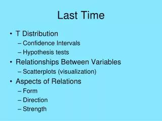
Last Time • T Distribution • Confidence Intervals • Hypothesis tests • Relationships Between Variables • Scatterplots (visualization) • Aspects of Relations • Form • Direction • Strength
Reading In Textbook Approximate Reading for Today’s Material: Pages 101-105 , 447-465, 511-516 Approximate Reading for Next Class: Pages 110-135, 560-574
Scatterplot E.g. Class Example 16: How does HW score predict Final Exam? xi = HW, yi = Final Exam • In top half of HW scores: Better HW Better Final
Important Aspects of Relations • Form of Relationship • Direction of Relationship • Strength of Relationship
I. Form of Relationship • Linear: Data approximately follow a line Previous Class Scores Example http://www.stat-or.unc.edu/webspace/courses/marron/UNCstor155-2009/ClassNotes/Stor155Eg16.xls Final vs. High values of HW is “best” • Nonlinear: Data follows different pattern Nice Example: Bralower’s Fossil Data http://www.stat-or.unc.edu/webspace/courses/marron/UNCstor155-2009/ClassNotes/Stor155Eg17.xls
Bralower’s Fossil Data http://www.stat-or.unc.edu/webspace/courses/marron/UNCstor155-2009/ClassNotes/Stor155Eg17.xls From T. Bralower, formerly of Geological Sci. Studies Global Climate, millions of years ago
II. Direction of Relationship • Positive Association X bigger Y bigger • Negative Association X bigger Y smaller Note: Concept doesn’t always apply: Bralower’s Fossil Data
III. Strength of Relationship Idea: How close are points to lying on a line? Revisit Class Scores Example: http://www.stat-or.unc.edu/webspace/courses/marron/UNCstor155-2009/ClassNotes/Stor155Eg16.xls
Comparing Scatterplots Additional Useful Visual Tool
Comparing Scatterplots Additional Useful Visual Tool: • Overlaying multiple data sets
Comparing Scatterplots Additional Useful Visual Tool: • Overlaying multiple data sets • Allows comparison
Comparing Scatterplots Additional Useful Visual Tool: • Overlaying multiple data sets • Allows comparison • Use different colors or symbols
Comparing Scatterplots Additional Useful Visual Tool: • Overlaying multiple data sets • Allows comparison • Use different colors or symbols • Easy in EXCEL (colors are automatic)
Comparing Scatterplots HW HW: 2.21, 2.25
III. Strength of Relationship Idea: How close are points to lying on a line? Revisit Class Scores Example: http://www.stat-or.unc.edu/webspace/courses/marron/UNCstor155-2009/ClassNotes/Stor155Eg16.xls
III. Strength of Relationship Idea: How close are points to lying on a line? Now get quantitative
Section 2.2: Correlation Main Idea: Quantify Strength of Relationship
Section 2.2: Correlation Main Idea: Quantify Strength of Relationship Context: • A numerical summary
Section 2.2: Correlation Main Idea: Quantify Strength of Relationship Context: • A numerical summary • In spirit of mean and standard deviation
Section 2.2: Correlation Main Idea: Quantify Strength of Relationship Context: • A numerical summary • In spirit of mean and standard deviation • But now applies to pairs of variables
Section 2.2: Correlation Main Idea: Quantify Strength of Relationship Specific Goals
Section 2.2: Correlation Main Idea: Quantify Strength of Relationship Specific Goals: • Near 1: for positive relat’ship & nearly linear
Section 2.2: Correlation Main Idea: Quantify Strength of Relationship Specific Goals: • Near 1: for positive relat’ship & nearly linear • > 0: for positive relationship (slopes up)
Section 2.2: Correlation Main Idea: Quantify Strength of Relationship Specific Goals: • Near 1: for positive relat’ship & nearly linear • > 0: for positive relationship (slopes up) • = 0: for no relationship
Section 2.2: Correlation Main Idea: Quantify Strength of Relationship Specific Goals: • Near 1: for positive relat’ship & nearly linear • > 0: for positive relationship (slopes up) • = 0: for no relationship • < 0: for negative relationship (slopes down)
Section 2.2: Correlation Main Idea: Quantify Strength of Relationship Specific Goals: • Near 1: for positive relat’ship & nearly linear • > 0: for positive relationship (slopes up) • = 0: for no relationship • < 0: for negative relationship (slopes down) • Near -1: for negative relat’ship & nearly linear
Correlation - Approach Numerical Approach
Correlation - Approach Numerical Approach: for symmetric around
Correlation - Approach Numerical Approach: for symmetric around has similar properties
Correlation - Approach Numerical Approach: for symmetric around has similar properties Worked out Example : http://www.stat-or.unc.edu/webspace/courses/marron/UNCstor155-2009/ClassNotes/Stor155Eg18-new.xls
Correlation – Graphical View Plots (a) & (b): illustrating : • > 0 for positive relationship
Correlation – Graphical View Plots (a) & (b): illustrating : • > 0 for positive relationship
Correlation – Graphical View Plots (a) & (b): illustrating : • > 0 for positive relationship • < 0 for negative relationship
Correlation – Graphical View Plots (a) & (b): illustrating : • > 0 for positive relationship • < 0 for negative relationship
Correlation – Graphical View Plots (a) & (b): illustrating : • Bigger for data closer to line
Correlation – Graphical View Plots (a) & (b): illustrating : • Bigger for data closer to line
Correlation – Graphical View But not all goals are satisfied
Correlation – Graphical View Problem 1: Not between -1 & 1
Correlation – Graphical View Problem 2: Feels “Scale”, see plot (c) (just 10 1 vertical rescaling of)
Correlation – Graphical View Problem 2: Feels “Scale”, see plot (c) (just 10 1 vertical rescaling of) ( feels factor of 1/10)
Correlation – Graphical View Problem 3: Feels “Shift” even more, see (d) (even gets sign wrong!)
Correlation – Graphical View Problem 3: Feels “Shift” even more, see (d) (even gets sign wrong!) • Data trend upwards
Correlation – Graphical View Problem 3: Feels “Shift” even more, see (d) (even gets sign wrong!) • Data trend upwards • But < 0
Correlation - Approach Solution to above problems
Correlation - Approach Solution to above problems: Standardize!
Correlation - Approach Solution to above problems: Standardize! Define Correlation
Correlation - Approach Solution to above problems: Standardize! Define Correlation
Correlation - Example Revisit above example http://www.stat-or.unc.edu/webspace/courses/marron/UNCstor155-2009/ClassNotes/Stor155Eg18-new.xls • r is always same, and ~1, for (a)
Correlation - Example Revisit above example http://www.stat-or.unc.edu/webspace/courses/marron/UNCstor155-2009/ClassNotes/Stor155Eg18-new.xls • r is always same, and ~1, for (a), (c)
Correlation - Example Revisit above example http://www.stat-or.unc.edu/webspace/courses/marron/UNCstor155-2009/ClassNotes/Stor155Eg18-new.xls • r is always same, and ~1, for (a), (c), (d)