Download
1 / 87
880 likes | 1.11k Vues
3.1 Introduction. In this chapter, we learn: Some facts related to economic growth that later chapters will seek to explain. How economic growth has dramatically improved welfare around the world. this growth is actually a relatively recent phenomenon. 3.1 Introduction.

E N D
3.1 Introduction • In this chapter, we learn: • Some facts related to economic growth that later chapters will seek to explain. • How economic growth has dramatically improved welfare around the world. • this growth is actually a relatively recent phenomenon
3.1 Introduction • In this chapter, we learn: • Some tools used to study economic growth, including how to calculate growth rates. • Why a “ratio scale” makes plots of per capita GDP easier to understand.
The United States of a century ago could be mistaken for Kenya or Bangladesh today. Some countries have seen rapid economic growth and improvements to health quality, but many others have not.
3.2 Growth over the Very Long Run • Sustained increases in standards of living are a recent phenomenon. • Sustained economic growth emerges in different places at different times. • Thus, per capita GDP differs remarkably around the world.
The Great Divergence The recent era of increased difference in standards of living across countries. Before 1700 Per capita GPD in nations differed only by a factor of two or three. Today Per capita GPD differs by a factor of 50 for several countries.
3.3 Modern Economic Growth • Timeline: from 1870 to 2000, United States per capita GDP . . . • . . . rose by nearly 15-fold. • Implications for you? • A typical college student today will earn a lifetime income about twice his or her parents.
3.4 Modern Growth around the World • After World War II, growth in Germany and Japan accelerated. • Convergence • Poorer countries will grow faster to “catch up” to the level of income in richer countries. • Brazil had accelerated growth until 1980 and then stagnated. • China and India have had the reverse pattern.
A Broad Sample of Countries • Over the period 1960–2007 • Some countries have exhibited a negative growth rate. • Other countries have sustained nearly 6 percent growth. • Most countries have sustained about 2 percent growth. • Small differences in growth rates result in large differences in standards of living.
Case Study: People versus Countries • Since 1960: • The bulk of the world’s population is substantially richer. • The fraction of people living in poverty has fallen. • A major reason for changes • Economic growth in China and India • These are 40 percent of the world population!
Case Study: Growth Rules in a Famous Example, Yt= AtKt1/3Lt2/3 • Applying rules of growth rates • Original output equation: • Use multiplication rule to get • Use exponent rule to get
3.6 The Costs of Economic Growth • The benefits of economic growth • Improvements in health • Higher incomes • Increase in the variety of goods and services
Costs of economic growth include: • Environmental problems • Income inequality across and within countries • Loss of certain types of jobs • Economists generally have a consensus that the benefits of economic growth outweigh the costs.
3.7 A Long-Run Roadmap • Are there certain policies that will allow a country to grow faster? • If not, what about a country’s “nature” makes it grow at a slower rate?
Summary • Sustained growth in standards of living is a very recent phenomenon. • If the 130,000 years of human history were warped and collapsed into a single year, modern economic growth would have begun only at sunrise on the last day of the year.
Summary • Modern economic growth has taken hold in different places at different times. • Since several hundred years ago, when standards of living across countries varied by no more than a factor of 2 or 3, there has been a “Great Divergence.” • Standards of living across countries today vary by more than a factor of 60.
Since 1870 Growth in per capita GDP has averaged about 2 percent per year in the United States. Per capita GDP has risen from about $2,500 to more than $37,000. Growth rates throughout the world since 1960 show substantial variation Negative growth in many poor countries Rates as high as 6 percent per year in several newly industrializing countries, most of which are in Asia
Growth rates typically change over time In Germany and Japan Growth picked up considerably after World War II. Incomes converged to levels in the United Kingdom. Growth rates have slowed down as this convergence occurred.
Brazil exhibited rapid growth in the 1950s and 1960s and slow growth in the 1980s and 1990s. China showed the opposite pattern.
Economic growth, especially in India and China, has dramatically reduced poverty in the world. In 1960 Two out of three people in the world lived on less than $5 per day (in today’s prices). By 2000 This number had fallen to only 1 in 10.
4.1 Introduction • In this chapter, we learn: • How to set up and solve a macroeconomic model. • How a production function can help us understand differences in per capita GDP across countries. • The relative importance of capital per person versus total factor productivity in accounting for these differences. • The relevance of “returns to scale” and “diminishing marginal products.” • How to look at economic data through the lens of a macroeconomic model.
A model: Is a mathematical representation of a hypothetical world that we use to study economic phenomena. Consists of equations and unknowns with real world interpretations. Macroeconomists: Document facts. Build a model to understand the facts. Examine the model to see how effective it is.
4.2 A Model of Production • Vast oversimplifications of the real world in a model can still allow it to provide important insights. • Consider the following model • Single, closed economy • One consumption good
Setting Up the Model • A certain number of inputs are used in the production of the good • Inputs • Labor (L) • Capital (K) • Production function • Shows how much output (Y) can be produced given any number of inputs
Others variables with a bar are parameters. Production function: Productivity parameter Output Inputs
The Cobb-Douglas production function is the particular production function that takes the form of Assumed to be 1/3. Explained later. • A production function exhibits constant returns to scale if doubling each input exactly doubles output.
Returns to Scale Comparison Find the sum of exponents on the inputs Result the function has constant returns to scale the function has increasing returns to scale the function has decreasing returns to scale • sum to 1 • sum to more than 1 • sum to less than 1
Standard replication argument A firm can build an identical factory, hire identical workers, double production stocks, and can exactly double production. Implies constant returns to scale.
Allocating Resources • The rental rate and wage rate are taken as given under perfect competition. • For simplicity, the price of the output is normalized to one. Firm chooses inputs to maximize profit Wage rate Rental rate of capital
The marginal product of labor (MPL) The additional output that is produced when one unit of labor is added, holding all other inputs constant. The marginal product of capital (MPK) The additional output that is produced when one unit of capital is added, holding all other inputs constant.
The solution is to use the following hiring rules: Hire capital until the MPK = r Hire labor until MPL = w
If the production function has constant returns to scale in capital and labor, it will exhibit decreasing returns to scale in capital alone.
Solving the Model: General Equilibrium • The model has five endogenous variables: • Output (Y) • the amount of capital (K) • the amount of labor (L) • the wage (w) • the rental price of capital (r)
The model has five equations: The production function The rule for hiring capital The rule for hiring labor Supply equals the demand for capital Supply equals the demand for labor The parameters in the model: The productivity parameter The exogenous supplies of capital and labor
A solution to the model A new set of equations that express the five unknowns in terms of the parameters and exogenous variables Called an equilibrium General equilibrium Solution to the model when more than a single market clears
In this model The solution implies firms employ all the supplied capital and labor in the economy. The production function is evaluated with the given supply of inputs. The wage rate is the MPL evaluated at the equilibrium values of Y, K, and L. The rental rate is the MPK evaluated at the equilibrium values of Y, K, and L.
Interpreting the Solution • If an economy is endowed with more machines or people, it will produce more. • The equilibrium wage is proportional to output per worker. • Output per worker = (Y/L) • The equilibrium rental rate is proportional to output per capital. • Output per capital = (Y/K)
In the United States, empirical evidence shows: Two-thirds of production is paid to labor. One-third of production is paid to capital. The factor shares of the payments are equal to the exponents on the inputs in the Cobb-Douglas function.