Game Playing in AI: Understanding Minimax Strategy and Search Problems
This overview delves into game theory as it applies to artificial intelligence, focusing on two-player, deterministic, and zero-sum games. It discusses the historical context of game-playing AI, highlighting achievements in games like Chess, Checkers, and Othello. The Minimax algorithm, which offers an optimal decision-making strategy against knowledgeable opponents, is explored, alongside issues of game complexity and the benefits of α-β pruning. Ultimately, the discussion illustrates the challenges and methodologies in developing AI for competitive gaming environments.

Game Playing in AI: Understanding Minimax Strategy and Search Problems
E N D
Presentation Transcript
6. Fully Observable Game Playing 2012/03/28
Game Theory • Studied by mathematicians, economists, finance • In AI, we limit game to • deterministic • turn-taking • two-player • zero-sum • perfect information • This means deterministic, full observable environments in which there are two agents whose action must alternate and in in which the utility values at the end of the game are always equal and opposite
Types of Games • Game playing was one of the first tasks undertaken in AI • Machines have surpassed humans on checker and Othello, have defeated human champions in chess and backgammon • In Go, computers perform at the amateur level
Game as Search Problems • Games offer pure, abstract competition • A chess playing computer would be an existence proof of a machine doing something generally thought to require intelligence • Games are idealization of worlds in which • the world state is fully accessible • the (small number of) actions are well-defined • uncertaintydue to moves by the opponent due to the complexity of games
Game as Search Problems (cont.-1) • Games are usually much too hard to solve • Example, chess: • average branching factor = 35 • average moves per player = 50 • total number of nodes in search tree = 35100 or 10154 • total number of different legal positions = 1040 • Time limits for making good decisions • Unlikely to find goal, must approximate
Game as Search Problems (cont.-2) • Initial State • How does the game start? • Successor Function • A list of legal (move, state) pairs for each state • Terminal Test • Determine when game is over • Utility Function • Provide numeric value for all terminal states • e.g., win, lose, draw with +1, -1, 0
Game Tree (2-player, deterministic, turns) Game tree complexity 9!=362880 Game board complexity 39= 19683
Minimax Strategy • Assumption • Both players are knowledgeable and play the best possible move • MinimaxValue(n) = Utility(n) if n is a terminal state maxsSuccessors(n)MinimaxValue(s) if n is a MAX node minsSuccessors(n)MinimaxValue(s) if n is a MIN node
Minimax Strategy (cont.) • Is a Optimal Strategy • Leads to outcomes at least as good as any other strategy when playing an infallible opponent • Pick the option that most (max) minimizes the damage your opponent can do • maximize the worst-case outcome • because your skillful opponent will certainly find the most damaging move
Minimax • Perfect play for deterministic, perfect information games • Idea: choose moves to a position with highest minimax value = best achievable payoff against best play
5 2 1 3 6 2 0 7 Minimax – Animated Example 3 6 The computer can obtain 6 by choosing the right hand edge from the first node. Max 6 Min 5 3 1 3 0 7 Max 6 5 13
function MINIMAX-DECISION(state) returns an action inputs: state, current state in game v MAX-VALUE(state) return the action in SUCCESSORS(state) with value v function MAX-VALUE(state) returns a utility value if TERMINAL-TEST(state) then return UTILITY(state) v – fora, sin SUCCESSORS(state) do v MAX( v, MIN-VALUE(s)) returnv function MIN-VALUE(state) returns a utility value if TERMINAL-TEST(state) then return UTILITY(state) v fora, sin SUCCESSORS(state) do v MIN(v, MAX-VALUE(s)) returnv Minimax Algorithm
Optimal Decisions in Multiplayer Games • Extend the minimax idea to multiplayer games • Replace the single value for each node with a vector of values
Minimax Algorithm (cont.) • Generate the whole game tree • Apply the utility function to each terminal state • Propagate utility of terminal states up one level Utility(n) = max / min (n.1, n.2, …, n.b) • At the root, MAX chooses the move leading to the highest utility value
Analysis of Minimax • Complete? Yes, only if the tree is finite • Optimal? Yes, against an optimal opponent • Time? O(bm), is a complete depth-first search m: max depth, b: # of legal moves • Space? O(bm), generate all successors at once or O(m), generate successor one at a time • For chess, b 35, m 100 for reasonable games Exact solution completely infeasible
Complex Games • What happens if minimax is applied to large complex games? • What happens to the search space? • Example, chess • Decent amateur program 1000 moves / second • 150 seconds / move (tournament play) • Look at approx. 150,000 moves • Chess branching factor of 35 • Generate trees that are 3-4 ply • Resultant play – pure amateur
- Pruning • The problem of minimax search • # of states to examine: exponential in number of moves • - pruning • return the same move as minimax would, but prune away branches that cannot possibly influence the final decision • – lower bound on MAX node, never decreasing • value of the best (highest) choice so far in search of MAX • – upper bound on MAX node, never increasing • value of the best (lowest) choice so far in search of MIN
[-, 2] 2 5 14 ? 2 5 14 ? - Pruning Example - 1 (2nd Ed.)
- Pruning (cont.) • cut-off • Search is discontinued below any MIN node with min-value • cut-off • Search is discontinued below any MAX node with max-value • Order of considering successors matters (look at step f in previous slide) • If possible, consider best successors first
max min max min - Pruning (cont.) • If n is worse than ,max will avoid it prune the branch • If m is better than n for player, we will never get to n in play and just prune it
6 = - = 6 = 6 = 6 6 2 6 8 2 5 = - 6 = = - 8 = 6 = - 6 = - Pruning Example - 2 = - = A = - = = 6 = B C = - = = - = 6 = 6 = D E F G H I J K L M L M 6 5 8 6 2 1 5 4
MAX a b c MIN d f g MAX e MIN 1 2 3 4 5 7 1 0 2 6 1 5 - Pruning Example - 3 Node Alpha Beta a -∞ ∞ Node Alpha Beta a 3 ∞ b -∞ 3 b -∞ ∞ d 1 ∞ d 2 ∞ d 3 ∞ d -∞ ∞ e 4 3 CUT-OFF e -∞ 3 c 3 ∞ c 3 3 CUT-OFF f 3 ∞ Completed
Key: -∞ = negative infinity; +∞ = positive infinity The last value in a square is the final value assigned to the specific variable, i.e. at the end of the search Node A’s a = 3.
function ALPHA-BETA-SEARCH(state) returns an action inputs: state, current state in game v MAX-VALUE(state, –, ) return the action in SUCCESSORS(state) with value v function MAX-VALUE(state, , ) returns a utility value inputs: state, current state in game , the value of the best alternative for MAX along the path to state , the value of the best alternative for MIN along the path to state if TERMINAL-TEST(state) then return UTILITY(state) v – fora, s in SUCCESSORS(state) do v MAX(v, MIN-VALUE(s, , )) ifvthen returnv// fail-high MAX(, v) returnv - Algorithm
- Algorithm (cont.) function MIN-VALUE(state, , ) returns a utility value inputs: state, current state in game , the value of the best alternative for MAX along the path to state , the value of the best alternative for MIN along the path to state if TERMINAL-TEST(state) then return UTILITY(state) v fora, s in SUCCESSORS(state) do v MIN(v, MAX-VALUE(s, , )) ifvthen returnv // fail low MIN(, v) returnv
MAX a MIN b c d e f g MAX h i j k l m n MIN MAX 7 4 2 5 5 1 0 2 8 7 3 0 1 2 - Pruning Example - 4
MAX a MIN b c d e f g MAX h i j k l m n o MIN MAX 5 1 1 2 0 -1 -5 0 -1 0 -4 -3 3 1 1 4 - Pruning Example - 5
Analysis of - Search • Pruning does not affect final result • The effectiveness of - pruning ishighly dependent on the order in which the successors are examinedIt is worthwhile to try to examine first the successors that are likely to be best • e.g., Example 1 (e,f) • If successors of D is 2, 5, 14 (instead of 14, 5, 2)then 5, 14 can be pruned
Analysis of - Search (cont.) • If best move first (perfect ordering), • the total number of nodes examined = O(bm/2) • effective branching factor = b1/2 • for chess, 6 instead 35i.e., - can look ahead roughly twice as far as minimax in the same amount of time • If random order, • the total number of nodes examined = O(b3m/4) for moderate b
Imperfect, Real-Time Decisions • No practical to assume the program has time to search all the ways to terminal states • Since moves must be made in a reasonable amount of time, to alter minimax or - in two ways • Evaluation Function (instead of utility function) • an estimate of the expected utility of game from a given position • Cutoff Test (instead of terminal test) • decide when to apply Eval • e.g., depth limit (perhaps add quiescence search)
Evaluation Functions • The heuristic that estimates expected utility • Preserve the ordering among terminal states in the same way as the true utility function,otherwise it can cause bad decision making • Computation cannot take too long • For nonterminal states, it should be strongly correlated with the actual chances of winning • Define features of game state that assist in evaluation • What are features of chess? e.g., # of pawns possessed, etc. • Weighted Linear Function • Eval(s) = w1f1(s) + w2f2(s) + … + wnfn(s)
Evaluation Functions (cont.-1) (a) Black has an advantage of a knight and two pawns and will win the game (b) Black will lose after white captures the queen
Evaluation Functions (cont.-2) • Digression: Exact values don’t matter • Behavior is preserved under any monotonic transformation of Eval • Only the order matter payoff in deterministic games acts as an order utility function
Cutting off Search • When do you use evaluation functions? ifCutoff-Test(state, depth)then returnEval(state) • controlling the amount of search is to set a fixed depth limit d • Cutoff-Test(state, depth) returns 1 or 0 • when 1 is returned for all depth greater than some fixed depth d, use evaluation function • cutoff beyond a certain depth • cutoff if state is stable (more predictable) • cutoff moves you know are bad (forward pruning) • Can have disastrous effect if evaluation functions are not sophisticated enough • Should continue the search until a quiescent position is found
Cutting off Search (cont.) • Does it work in practice? • bm = 106, b = 35 m = 4 • 4-ply lookahead is a hopeless chess player • 4-ply human novice • 8-ply typical PC, human master • 12-ply Deep Blue, Kasparov
Horizontal Effect a series of checks by the black rook forces the inevitable queening move by white “over the horizontal” and makes the position look like a win for black, when it is really a win for white • Horizontal effect arises when the program is facing a move by the opponent that causes serious damage and is ultimately unavoidable • At present, no general solution has been found for horizontal problem
Suggestion • Improve evaluation function • Know that the bishop is trapped • Make the search deeper • Make the search depth more flexible • Program searches deeper in the line that a pawn is being given away, and less deep in other lines
HW2, Deadline 4/12 • Design the Evaluation Functions for Chinese chess and Chinese Dark chess.