Download
1 / 12
120 likes | 145 Vues
This study focuses on assimilating GPS data into kinematic fault models for Bungo Channel and Cascadia events, analyzing slip rates, stress drops, and seismic activities. The paper discusses the Extended Kalman Filter, State Transition Equation, and data smoothing techniques used in fault modeling.

E N D
Assimilation of Continuous GPS Data into Kinematic Fault Models Jeff McGuire1, Paul Segall2, and Shin’ichi Miyazaki3 1 Woods Hole Oceanographic Institution 2 Stanford University 3 ERI, University of Tokyo
1996-1998 Bungo Channel Aseismic Slip Transient Time (yr)
Observation Equation x: Antenna Position Vs: Secular Velocity s: Transient Fault slip L: Benchmark Wobble f(t): Reference Frame error e: estimation error
State Vector at Measurement Epoch K Fault Slip Benchmark Wobble Reference Frame Smoothing Parameters
Observation equation: • Separates spatially coherent signals from local ones • Enforces positivity of slip-rate • Enforces a spatially smooth solution State Transition Equation: Current Fault Slip Model: • Encorporates random walk model of benchmark motion and slip-rate
Extended Kalman Filter A Priori Estimate Backsmoothed Estimate Prediction: Residual Update
Bungo Channel Event Summary • Up to ~.6 m of slip over 1 year between depths of 30-60 km • The Bungo channel event started about 1 month after the 2nd Hyuganada earthquake • There was no propagation between the Hyuga-nada earthquake afterslip and the Bungo channel event • The average stress-drop was about .15 M Pa (~1/10th of a ordinary earthquake) • A previously unidentified, Mw ~6.5 event occurred in • mid 1997 in the Hyuga-nada area
Displacement (mm) Time from 1999.5 to 1999.9
1999 Cascadia Event Summary • Slip-Pulse like propagation with a centroid velocity of ~5 km/day • Mw ~ 6.9 • Maximum slip of ~ 6 cm • Slip confined between about 25 and 40 km depth • Average Stress Drop of about .015 M Pa • Stress Changes on the order of 10-5 * lithostatic drive rupture propagation over distances of ~200 km.
The Network Inversion Filter and ACES • Monitor the bottom boundary of the seismogenic zone • Test constituitive laws for the aseismic region of faults just below the seismogenic zone. • Encorporate a true dynamic model for xk+1=t(xk) • -At what spatial/temporal scales does information about aseismic slip-rate become useful?