Non-Linear and Smooth Regression
120 likes | 249 Vues
This document provides a comprehensive overview of non-linear and smooth regression methods, emphasizing non-linear parametric models. It includes a practical example using the nls function in R to model the relationship between pressure (P) and volume (V) based on Boyle's law data. The document explores polynomial fits, smoothing splines, and lowess for data smoothing. Additionally, it touches on DOSE RESPONSE MODELS and mixed-effects models, illustrating their applications in various data scenarios, including orthodontic measurements over time.

Non-Linear and Smooth Regression
E N D
Presentation Transcript
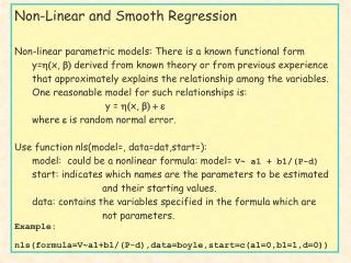
Non-Linear and Smooth Regression Non-linear parametric models: There is a known functional form y=x, derived from known theory or from previous experience that approximately explains the relationship among the variables. One reasonable model for such relationships is: y = x, where is random normal error. Use function nls(model=, data=dat,start=): model: could be a nonlinear formula: model= V~ a1 + b1/(P-d) start: indicates which names are the parameters to be estimated and their starting values. data: contains the variables specified in the formula which are not parameters. Example: nls(formula=V~a1+b1/(P-d),data=boyle,start=c(a1=0,b1=1,d=0))
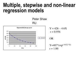
Boyle Data: P x V = cte. V P 29.750 1.0 19.125 1.5 14.375 2.0 9.500 3.0 7.125 4.0 5.625 5.0 4.875 6.0 4.250 7.0 3.750 8.0 3.375 9.0 3.000 10.0 2.625 12.0 2.250 14.0 2.000 16.0 1.875 18.0 1.750 20.0 1.500 24.0 1.375 28.0 1.250 32.0 boyle <- data.frame(matrix(scan(,ncol=2,byrow=T)) names(boyle) <- c("V","P") attach(boyle) par(mfrow=c(2,2),cex=1.07,mar=c(4,4,0.2,0.2),mgp=c(2,1,0)) plot(P,V,pch=16,col=2) # Plot 1 plot(log(P),log(V),pch=16,col=2) # Plot 2 lsfit(log(P),log(V))$coef [1] 3.2717004 -0.9152016 The slope is close to -1. Pm1 <- 1/P rm1 <- lsfit(Pm1,V) plot(rm1$resid,V,pch=16,col=2) # Plot 3 See U-pattern. It shows a possible quadratic fit. rm2 <- lsfit(cbind(Pm1,Pm1^2),V) plot(rm2$resid,V,pch=16,col=2) # Plot 4 The Residuals look very good!! We have obtained the fit: V= a + b 1/P + c (1/P)^2, where a , b and c are rm2$coef [1] 0.4127083 26.0636703 3.2543654
The polynomial in the equation looks like a Taylor expansion of something A possibility will be to expand 1/(P-d) as a polynomial on 1/P around 0. Then we get 1/(P-d) = 1/P + d (1/P)^2 + d^2 (1/P)^3 + O( (1/P)^4 ) So , Fit 1 suggests a possible fit ( Fit 2) V = a1 + b1 1/(P -d) where a1 = a = 0.41 , d = c/b = 0.12, and b1=26.06 nls(formula= V~ a1 + b1/(P-d),data=boyle, start=c(a1=0,b1=1,d=0)) Nonlinear regression mo1del model: V ~ a1 + b1/(P - d) data: boyle a1 b1 d 0.4016758 26.2392374 0.1055646 • residual sum-of-squares: 0.05783763 # We conclude d= 0.1055646 par(mfrow=c(2,2)) d <- 0.1055646 rmd1 <- lsfit(1/(P-d),V) d <- 0.12 rmd2 <- lsfit(1/(P-d),V) plot(P,rmd1$resid,pch=16,col=2) plot(P,rmd2$resid,pch=16,col=2) • boxplot(rmd1$resid,rm2$resid,rmd2$resid,rm1$resid)
Smoothing Regression Polynomial fits: Not so great. Smoothing Splines: The method of smoothing splines consists of dividing the domain of x in K+1 regions by the ordered points t1,…,tk, and consider the basis functions {1, x, x2, {x-t1}+3 , …… , {x-tk}+3} = {Bi(x)} where the ai’s are fitted by least squares. spl <- function(x,y,p=10){ xx = unique(quantile(x,c(0:(p-1))/(p-1))) p = length(xx) x = c(seq(from=min(x),to=max(x),length=200),x) z = cbind(x,x^2) for(i in 1:(p-1)) z <- cbind(z, pmax(x-xx[i],0)^3) yy <- data.frame(y=y ,z[-(1:200),]) ff= predict(xlm<-lm(y~.,data=yy),data.frame(z[(1:200),])) plot(x[-(1:200)],y) lines(x[1:200],ff) list(x=x,y=predict(xlm)) }
Lowess: Locally linear model The smoothing parameter is f= fraction of the data that is used in each locally linear fit. Lowess is easy to generalize to high dimensions z <- spl(x,y) lines(lowess(x,y),col=2) lines(smooth.spline(x,y),col=3)
DOSE RESPONSE MODELS: EMAX model: 4 params: R = E0 + EMAX Dl /(ED50l + Dl ) + Error 3 params: R = E0 + EMAX D /(ED50 + D ) + Error Estimate using maximum likelihood drd = read.table("drd.txt") m = nls(y~e0 +(emax * dose)/(dose+ed50), start= c(ed50=2, e0=1,emax=31),control=nls.control(maxiter=100),trace=TRUE,na.action=na.omit,data=drd) m1 = nls(y~e0 +(emax * dose^lambda)/(dose^lambda+ed50^lambda), start= c(ed50=2, e0=1,emax=31,lambda=1),control=nls.control(maxiter=100),trace=TRUE,na.action=na.omit,data=drd) m2 = nls(y~e0 +(emax * (dose)^lambda), start= c( e0=2.4,emax=10,lambda=1),control=nls.control(maxiter=100),trace=TRUE,na.action=na.omit,data=drd)
Mix effect models. Fixed effects + Random Effects Orthodont: change in an orthdontic measurement over time for several subjects. Distance: a numeric vector of distances from the pituitary to the pterygomaxillary fissure (mm). These distances are measured on x-ray images of the skull. Age: a numeric vector of ages of the subject (yr). Subject: an ordered factor indicating the subject on which the measurement was made. M01 to M16 for the males and F01 to F13 for the females. Sex: a factor with levels Male and Female Orth.new <- groupedData( distance ~ age | Subject, data = as.data.frame( Orthodont ), FUN = mean, outer = ~ Sex, labels = list( x = "Age", y = "Distance from pituitary to pterygomaxillary fissure" ), units = list( x = "(yr)", y = "(mm)") ) plot( Orth.new ) m1 <- lme(distance ~ age, data = Orthodont) m2 <- lme(distance ~ age + Sex, data = Orthodont, random = ~ 1) summary(m1) summary(m2)
Bayesian models Software: Winbugs http://www.mrc-bsu.cam.ac.uk/bugs/winbugs/contents.shtml Need data file and program file MCMC methods a. Suppose that we have a model for which we know the full joint distribution of all quantities. b. We want to sample values of the unknown parameters from their conditional (posterior) given the data (observed values) c. Gibbs sampling's basic idea: successively sample from the conditional distribution of each variables given all the other. d. Metropolis-within-Gibbs algorithm: appropriate for dificult full conditionals and does not necessarily generate a new value at each iteration e. Under broad conditions this process eventually provides samples from the joint posterior distribution of the unknown variables.
Winbugs Example: EMAX model model{ for (i in 1:N) { y[i] ~ dnorm(emx[i], tau) emx[i] <- e0 + (emax*pow(dose[i],lambda))/(pow(ed50,lambda)+pow(dose[i],lambda)) } e0 ~ dunif(0,10) tau ~ dgamma(0.01,0.001) emax ~ dunif(0,30) ed50 ~ dunif(0,120) lambda ~ dunif(0.01,3) sigma <- 1/sqrt(tau) }
list(dose = c(50, 50, 25, 5, 100, 0, 25, 0, 100, 100, 0, 50, 100, 5, 50, 25, 25, 0, 50, 0, 25, 0, 50, 25, 100, 100, 5, 5, 100, 25, 5, 0, 50, 25, 100, 50, 25, 0, 5, 0, 5, 100, 0, 25, 25, 100, 50, 100, 5, 0, 50, 25, 25, 50, 100, 5, 100, 5, 0, 50, 5, 0, 25, 25, 100, 50, 100, 5, 0, 50, 0, 5, 50, 0, 25, 100, 5, 50, 25, 25, 0, 5, 0, 100, 50, 5, 25, 25, 100, 5, 0, 0, 100, 5, 50, 50, 5, 50, 50, 50, 25, 0, 100, 25, 0, 5, 5, 50, 0, 25, 100, 5, 25, 5, 0, 50, 50, 100, 0, 5, 0, 25, 100, 25, 100, 50, 5, 50, 25, 50, 50, 5, 5, 25, 100, 0, 0, 50, 50, 100, 100, 5, 5, 25, 25, 0, 0, 0, 50, 100, 25, 5, 0, 25, 50, 100, 100, 5, 25, 50, 5, 0, 100, 0, 50, 25, 100, 50, 25, 5, 5, 100, 50, 100, 25, 100, 25, 50, 0, 0, 5, 5, 25, 100, 50, 50, 0, 5, 0, 5, 25, 100, 50, 25, 0, 0, 5, 50, 5, 100, 25, 0, 100, 25, 50, 25, 100, 5, 0, 5, 50, 50, 25, 5, 50, 100, 0, 25, 5, 100, 0, 5, 0, 25, 50, 100, 100, 5, 50, 25, 50, 5, 100, 25, 50, 100, 5, 25, 0, 50, 100, 5, 5, 0, 25, 50, 25, 100, 50, 5, 25, 25, 50, 0, 100, 100, 0, 5, 5, 25, 25, 50, 0, 0, 100, 5, 0, 100, 100, 5, 50, 5, 50, 25, 25, 0, 0, 5, 25, 0, 100, 5, 50, 50, 100, 25, 25, 0, 50, 5, 100, 50, 100, 5, 25, 0, 0, 0, 25, 25, 100, 5, 50, 50, 100, 50, 0, 25, 100, 5, 5, 50, 0, 100, 25, 25, 5, 50, 0, 5, 50, 25, 100, 0, 50, 5, 0, 25, 25, 0, 50, 5, 100, 100, 5, 5, 0, 100, 50, 25, 0, 100, 100, 25, 50, 50, 5, 0, 0, 5, 25, 25, 5, 50, 0, 0, 100, 5, 100, 50, 50, 100, 100, 25, 5, 0, 0, 5, 25, 0, 0, 100, 25, 5, 50, 50, 100, 25, 5, 100, 50, 0, 5, 25, 5, 100, 50, 0, 25, 5, 25, 50, 100, 25, 100, 50, 5, 0), y = c(-2, 21, 19, 7, 28, 0, 18, 1, -11, 18, 0, 11, 8, 4, 5, 7, 7, 0, -1, -3, 3, -6, -5, 3, 8, 26, 0, 4, 10, 2, 0, -1, 23, 7, 23, 3, 26, 6, -3, -3, -1, 1, 0, 11, 5, 18, -3, 18, 11, 3, 2, 9, -6, 13, 5, 12, 11, -4, 0, 24, 5, -8, 0, 0, 2, 3, 6, 3, 0, 7, 11, 9, -3, 1, 5, -2, 7, 0, 6, 0, 6, 1, -2, 0, 12, 2, 0, 9, 17, 12, 2, 6, 5, 11, 0, 9, 12, -3, 5, 16, 7, 0, 18, 7, -2, -2, 10, 14, -2, 12, -2, 1, 1, 9, 0, 24, 1, 28, 10, 2, 4, 5, 8, -6, 22, 21, 1, 5, 7, 7, -4, 16, 12, 8, 7, 10, -7, -3, -4, 1, 14, 2, -4, -2, 20, -1, 1, 0, 24, 19, 14, 2, 0, 0, -2, 22, 20, 16, -1, 15, 5, 18, 11, 4, 6, 9, 2, 19, 6, -2, 5, 0, 17, 3, 1, 24, 0, 10, 18, 4, 0, 5, -3, 15, 12, 13, 6, 5, 5, -6, -13, 5, 6, 1, 5, 22, 17, 5, -8, 17, 5, 0, 20, 14, 15, 4, 28, 12, 0, 4, -1, 4, 0, -5, 26, 2, -3, 0, 2, 3, 2, 18, 0, 21, -2, 25, 0, -3, 15, 18, 24, 1, 12, 21, 10, 29, 8, -1, -2, 7, 11, 8, 15, 7, 6, 1, 21, 19, -5, 5, 2, 7, 3, -6, 18, 0, 1, 1, 2, 1, -3, 5, 20, 0, -4, -1, -2, 7, 24, 5, 12, 13, 2, 21, 7, -2, -4, 6, 2, 4, 12, 0, 9, -5, 23, 3, 4, -13, 3, 13, 15, 6, 20, 3, 18, -3, 5, -1, 13, 0, 8, 6, 22, 22, 19, 22, -3, 10, 19, 4, 1, 0, 8, 12, 4, 8, 0, 21, 4, 19, 20, 18, 11, 5, 22, 6, -5, 17, 22, -1, 21, 13, 20, 18, 7, -7, 5, 7, 9, 3, -3, 23, 12, 28, 6, 8, -6, 0, 0, 0, -3, -2, -7, 18, -4, 20, 2, 0, 2, 6, 7, 1, 24, 6, 5, -2, 3, 7, 1, 0, -6, 7, 11, -1, 25, 1, 12, -4, 0, 10, -2, 0, 4, -2, 15, 1, 3, 9, 6, -2, 1, 1, 2, 18, 2, 5, 2, 2), N=396)