Hypothesis Testing
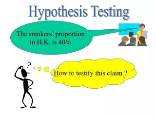
How to testify this claim ?. Hypothesis Testing. The smokers’ proportion in H.K. is 40%. Hypothesis Testing. The smokers’ proportion in H.K. is 40%. What kind of hypothesis ?. Statistical hypothesis. assumption about parameter of population, e.g.

Hypothesis Testing
E N D
Presentation Transcript
How to testify this claim ? Hypothesis Testing The smokers’ proportion in H.K. is 40%.
HypothesisTesting The smokers’ proportion in H.K. is 40%. What kind of hypothesis ? Statisticalhypothesis assumption about parameter of population, e.g. It’s impractical to investigate the whole population, we just select a sample and base on the information yielded to performtesting. This kind of testing is called
We write H0 : p = 0.5 H1 : p 0.5 “null” means nothing, for this e.g., the coin is fair, nothing special. Two kinds of Hypothesis John: The coin I am holding is fair. May: I don’t believe. I want to test. Let p = probability that obtaining a head. We have two kinds of hypothesis. (1) The coin is fair, p = 0.5. (2) The coin is not fair, p 0.5. is called the null hypothesis. is called the alternative hypothesis. Denoted as H0 Denoted as H1
Two-tailed test One-tailed test One-tailed test H0 : = 0 H1 : 0 H0 : = 0 H1 : > 0 H0 : = 0 H1 : < 0 Two kinds of Testing OR
What’s the relation betweenandzc ? Decision making Estimate: a sample parameter to estimate that of population. e.g. sample mean is an estimate for population mean. In AL, we need to test involving normal distribution only. Henceestimate is normally distributed in A.L. in general. Test statisticz = z ~ N(0,1) Before testing, choose a level of significance, For this level of significance, we can find a corresponding critical value zc.
N(0,1) /2 /2 zc zc N(0,1) N(0,1) zc zc For One-tailed Test OR H0: = 0 H1: < 0 H0: = 0 H1: > 0 For Two-tailed Test H0: = 0 H1: 0 If the test statistic lies in the shaded region, we rejectH0, otherwise, accept.
Test about mean Test statistic z = The test is OK if population data has normal distribution and any sample size, OR population data has any distribution and sample size is large, (n > 30)
z N(0,1) zc E.g. 39 Given : I.Q. of children is H.K. ~ N(100,20). A group of 62 children has mean I.Q. = 102.6. Is the sample group more intelligent than population? Given (significance level) = 0.05 Let x be the sample mean, then We want to test whether the group is more intelligent or not. The null hypothesis is: the group is nothing special! In symbol, H0: x = 100 The alternative hypothesis is: the group is more intelligent! In symbol, H1: x > 100 This is a one-tailed test Estimate = 102.6 Test statistic z = = 1.02 = 0.05 By table, zc = 1.645 Since 1.02 < 1.645, i.e. The test statistic z doesn’t lie in shaded region! Conclusion: we accept H0 at a significance level of 0.05 Caution: we are NOT saying that H0 is true!!
N(0,1) /2 /2 zc zc z E.g. 41 A lathe is adjusted so that dimension mean = 20 cm. A sample of 40 is selected and sample mean = 20.1 cm and s.d. = 0.2 cm. Do the results, test at 0.05 significance level, indicate that the machine is out of adjustment ? Let x = sample mean, then H0 : x= 20 H0 : the machine is nothing special, not out of adjustment. H1 : x 20 H1 : the machine is special, it is out of adjustment. This is a two-tailed test Estimate = 20.1 Test statistic z = = 3.16 = 0.05 By table, zc = 1.96 Since 3.16 > 1.96, i.e. The test statistic z does lie in shaded region! Conclusion: we reject H0 at a significance level of 0.05 Caution: we are NOT saying that H0 is untrue!!
A B The sample selected is ordinary. z doesn’t lie in extreme regions, indicating that the true mean is (>0) i.e. the mean = 0 is untrue, i.e.H0 is false! You’re lucky! z has small chance to lie in the region and you got it. However, the mean = 0 may be true, i.e. H0 may be true! N(0,1) /2 /2 zc zc N(,1) z z Reject H0 H0 is false x is a random variable, so is the test statistic z. The test statistic z is normally distributed. Hence z can lie on any region in (,) z lies in the “rejecting region”, either OR In hypothesis testing, we adopt the concept B.
E.g. 46 In a chemical plant the acid content of the effluent from the factory is measured frequently. From 400 measurements the acid content in gram per 100 liters of effluent is recorded in the following frequency distribution. Acid content 12 13 14 15 16 Frequency 5 52 235 74 34 (a) Find the mean acid content and the standard error of the mean. = 14.2 s = 0.815 s.e. = (b) Assuming a normal distribution of acid content, give 95% confidence limits for the mean acid content of the effluent. 95% confidence limits for mean are = 14.12 and 14.28
(c) Is the result consistent with a mean acid content of 14.13 g per 100 litres obtained from tests over several years ? N(0,1) /2 /2 zc zc z H0 : = 14.13 H1 : 14.13 This is a two-tailed test Estimate = 14.2 Test statistic z = = 1.72 = 0.05 By table, zc = 1.96 Since 1.72 < 1.96, at a significance level of 0.05 Conclusion: we accept H0 Hence at 5% significant level, the result is consistent. Caution: The level of significance must be stated! It’s meaningless in saying accept or reject H0 alone.
Test about proportion Test statistic z = The test is OK if sample size is large (n 30), np 10 and nq 10 and for small sample size, use binomial. in calculation of Ps, continuity correction must be made in passing from discrete to continuous variable.
Sample size = n Success no. = m Ps = m/n H1 : p > p0 adjusted Ps = (m0.5)/n H1 : p < p0 adjusted Ps = (m+0.5)/n Continuity Correction Believe me, I’ll tell you why later.
z N(0,1) zc E.g. 48 Last month unemployed rate = 7.1 %. This month, someone discovers 350 are unemployed in a random sample of 5000. Has the unemployment decreased this month ? = 0.05 H0 : p = 7.1% H1 : p < 7.1% Ps = = 0.0701 (Continuity correction) Test statistic z = = 0.248 Since 0.248 > 1.645, = 0.05 By table, zc = 1.645 we accept H0 at 5% level of significance. i.e. No change in unemployment rate this month.
Ps = = 0.895 z N(0,1) zc E.g. 49 A standard medication reduces pain in 80% of patients treated. A new medication for the same purpose produces 90 patients relieved among the first 100 tested. Does this new medication relieve more patients than before ? ( = 1%) H0 : p = 80% H1 : p > 80% zc = 2.33 = 0.01 > zc Test statistic z = = 2.375 Thus, reject H0 at 1% level of significance. i.e. New medication relieves more patients than before.
> 2.33 z N(0,1) zc E.g. 53 A manufacturer claims that less than 2% of the women use his birth control pill suffer from side effects. We have a feeling that this estimate is too low. We decide to test his claim at the 0.01 significance level using a sample of 900 randomly selected women. Find the decision rule. Let p = probability that a randomly selected user has side effect. H0 : p = 2% H1 : p > 2% = 0.01 zc = 2.33 z = For rejecting H0, set z > zc, yielding Ps > 0.0309 Let m = no. of “side effect” users in the sample, then m > 28.3 Hence the rule is: if there are more than 28 “side effect” users, we say that the claimed rate is too low, otherwise, fail to reject the claim.
E.g. 55 John tells you that he can control the tosses of fair coin. To see if he is right you take two ordinary coins and give him one. You toss one and ask him to toss the same thing. You repeat this experiment 18 times and John succeeds in tossing the same as you 15 times. Is John usual ? = 0.05. Let p = probability that tossing the same as you. Note: we use binomial instead. Note: the no. of trials = 18 is too small to use normal distribution. H0 : p = 0.5 H1 : p > 0.5 P(15 or above success) = (0.5)18[18C15 + 18C16 + 18C17 + 18C18] = 0.0038 < 0.05 (The chance of having 15 or more success is very small!) Conclusion: John is usual at 0.05 significance level.
P(X) . . . X n-2 n-1 n = 0.01 E.g. 57 A coin which is tossed n times comes up heads n times. What’s the min. n for which we can conclude at 0.01 significance level that the coin is not fair ? Consider two cases: one-tailed and two-tailed. Let p = probability of getting head in each toss. One-tailed test X = no. of heads in n tosses, then X~ B(n,0.5) H0 : p = 0.5 H1 : p > 0.5 n heads turn up. And we want to reject H0 at = 0.01 X = n should lie in the rejecting region. Thus P(X = n) < 0.01 min. n =7. min. n =8. Similarly, for Two-tailed test, we set
H0 : p = p0 H1 : p > p0 Remarks On Continuity Correction For one-tailed testing about proportion. We consider sample size n with no. of success X. Suppose that in a sample, we find m success out of n. To decide whether we reject H0 or not, we look into the chance that X is m or above, see whether this chance is too small. (i.e. less than or not.) Hence we concern P(X m) X is discrete and if we use continuous variable to approximate it, continuity correction must be carried out. P(X m) = That’s why we use the adjusted sample proportion (m0.5)/n as the test statistic instead of m/n. Try to “prove” the case for H1 : p < p0 on your own.
Sorry for the hurry lessons and I haven’t got much time on preparing these slides, please read the following on you own: E.g. 58, 61, 63, 65 Please do the following as your class work/ homework: 3(c) 4, 9, 11, 15, 22, 24, 26, 28, 31, 33, 36, 39 3(d) 1, 2, 3, 4, 17, 19, 25, 26, 27, 28, 34, 39 Bye.

