Chapter 6 – 2D Viewing

1. Chapter 6 – 2D Viewing

2. Co-ordinate Systems. • Cartesian – offsets along the x and y axis from (0.0) • Polar – (r,) • Graphic libraries mostly using Cartesian co-ordinates • Any polar co-ordinates must be converted to Cartesian co-ordinates • Four Cartesian co-ordinates systems in computer Graphics. • Modeling co-ordinates • World co-ordinates • Normalized device co-ordinates • Device co-ordinates

3. Modeling Co-ordinates • Also known as local coordinate. • Ex: where individual object in a scene within separate coordinate reference frames. • Each object has an origin (0,0) • So the part of the objects are placed with reference to the object’s origin.

4. World Co-ordinates • The world coordinate system describes the relative positions and orientations of every generated objects. • The scene has an origin (0,0). • The object in the scene are placed with reference to the scenes origin. • World co-ordinate scale may be the same as the modeling co-ordinate scale or it may be different.

5. Normalized Device Co-ordinates • Output devices have their own co-ordinates. • Co-ordinates values: The x and y axis range from 0 to 1 • All the x and y co-ordinates are floating point numbers in the range of 0 to 1 • This makes the system independent of the various devices coordinates. • This is handled internally by graphic system without user awareness.

6. Device Co-ordinates • Specific co-ordinates used by a device. • Pixels on a monitor • Points on a laser printer. • mm on a plotter. • The transformation based on the individual device is handled by computer system without user concern.

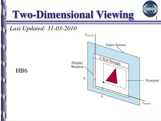
7. Two-Dimensional Viewing • Window: • A world-coordinate area selected for display. • Window defines what is to be viewed • Viewport: • An area on a display device to which a window is mapped. • Viewport defines where it is to be displayed • Viewing transformation: • The mapping of a part of a world-coordinate scene to device coordinates. • Most of the time, windows and viewports are usually rectangles in standard position(i.e aligned with the x and y axes). • In some application, others such as general polygon shape and circles are also available • However, other than rectangle will take longer time to process.

8. Window and viewports

9. Viewing Transformation • In 2D (two dimensional) viewing transformation is simply referred as the window-to-viewport transformationor the windowing transformation. • Mapping a window onto a viewport involves converting from one coordinate system to another. • If the window and viewport are in standard position, this just involves translation and scaling. • If the window and/or viewport are not in standard, then extra transformation which is rotation is required.

10. Window-To-Viewport Coordinate Transformation The sequence of transformations are: Translate the window to the origin Scale it to the size of the viewport Translate the scaled object to the position of the viewport.

11. Window-To-Viewport Coordinate Transformation

12. Viewing Transformation y-world y-view window window 1 x-view 0 1 x-world World and Viewport Normalised device

13. Window-To-Viewport Coordinate Transformation Window-to-Viewport transformation

14. . Window-To-Viewport Coordinate Transformation xv - xvmin = xw - xwmin xvmax - xvminxwmax - xwmin yv – yvmin = yw - ywmin yvmax – yvminywmax - ywmin From these two equations we derived xv = xvmin+ (xw – xwmin)sx yv = yvmin+ (yw – ywmin)sy where the scaling factors are sx = xvmax – xvminsy = yvmax - yvmin xwmax – xwminywmax - ywmin YWmax YVmax xw,yw xv,yv YWmin YVmin XVmax XVmin XWmin XWmax

15. Window-To-Viewport Coordinate Transformation • Relative proportions of objects are maintained if the scaling factors are the same (sx = sy). • Otherwise, world objects will be stretched or contracted in either x or y direction when displayed on output device.

16. The Viewing Pipeline

17. The Viewing Pipeline

18. Viewport-to-Normalized Device Coordinate Transformation • From normalized coordinates, object descriptions can be mapped to the various display devices. • When mapping window-to-viewport transformation is done to different devices from one normalized space, it is called workstation transformation.

19. Clipping • Clipping is a process of dividing an object into visible and invisible positions and displaying the visible portion and discarding the invisible portion. • Generally we have clipping algorithms for the following primitive types. • Point clipping • Line clipping • Area clipping (Polygon)

20. Clipping Window Viewport World Coordinates The clipping window is mapped into a viewport. Viewport Coordinates

21. Point Clipping For a point (x,y) to be inside the clip rectangle:

22. Line Clipping Cases for clipping lines

23. Line Clipping Cases for clipping lines

24. Line Clipping Cases for clipping lines

25. Line Clipping Cases for clipping lines

26. Line Clipping Cases for clipping lines

27. Line Clipping Cases for clipping lines

28. Cohen-Sutherland line clipping algorithm • This is one of the most popular line clipping algorithms. • This was introduced by Dan Cohen and Ivan Sutherland. • It was designed not only to find the endpoints very rapidly but also to reject even more rapidly any line that is clearly invisible. • This makes it a very good algorithm.

29. Cohen-Sutherland line clipping algorithm • Assign a four bit code to all regions. • Every line end point in a picture is assigned a 4-bit binary code known as region code. • That identifies the location of the point relative to the boundaries of the clipping rectangle. • Each bit position in the region code is used to indicate one of the 4 rectangle coordinates positions of the point with respected to clipping window to the left, right, below and top.

30. Cohen-Sutherland Clipping-Region Outcodes 1001 1000 1010 0001 0000 0010 0100 0110 0101

31. Cohen-Sutherland line clipping algorithm • Bit 1 – left • Bit 2 – right • Bit 3 – below • Bit 4 – top • A value of 1 in any bit position indicates that the point is in the relative position otherwise the bit position is set to zero. • If a point is within the clipping the region code is 0000.

32. Cohen-Sutherland line clipping algorithm • If the code of both the endpoints are 0000 then the line is totally visible and hence draw the line. • Bit values in the region codes are determined by comparing endpoint co-ordinate values (x, y) to the clip boundaries.

33. Cohen-Sutherland line clipping algorithm • Bit 1 is set to 1 if x < Xwmin • The other three bit values can be determined using similar comparison or calculating differences between endpoint co-ordinates and clipping boundaries. • Use the resultant sign of each differences calculation to set the corresponding value in the region code.

34. Cohen-Sutherland line clipping algorithm • Bit 1 is the sign bit of x-xwmin • Bit 2 is the sign bit of xwmax-x • Bit 3 is the sign bit of y-ywmin • Bit 4 is the sign bit of ywmax-y • If any line have 1 in the same bit position in the region codes for each endpoint are completely outside the clipping rectangle, so we discard the line

35. Cohen-Sutherland line clipping algorithm • For a line with end points co-ordinates (x1, y1) and (x2, y2) then the y coordinate of the intersection point with a vertical boundary can be obtained with the calculation • y=y1 + m(x-x1) (1) • Where the x value is set either to xwmin or xwmax.

36. Cohen-Sutherland line clipping algorithm • Similarly if we are looking for the intersection with a horizontal boundary, the x co-ordinate can be calculated as • x = x1 + 1/m (y-y1)  (2) • where y set either ywmin or ywmax.

37. Cohen-Sutherland Clipping Trivial Acceptance: O(P0) = O(P1) = 0 1001 1000 1010 P1 0001 0000 0010 P0 0100 0110 0101

38. Cohen-Sutherland Clipping: Trivial Rejection: O(P0) & O(P1)  0 P0 1001 1000 1010 P1 P0 0001 0000 0010 P0 P1 P1 0100 0110 0101

39. Cohen-Sutherland Clipping:O(P0) =0 , O(P1)  0 1001 1000 1010 P0 0001 0000 0010 P1 P1 P0 P0 0100 0110 0101 P1

40. Cohen-Sutherland Clipping: The Algorithm • Compute the outcodes for the two vertices • Test for trivial acceptance or rejection • Select a vertex for which outcode is not zero • There will always be one • Select the first nonzero bit in the outcode to define the boundary against which the line segment will be clipped. • Compute the intersection and replace the vertex with the intersection point • Compute the outcode for the new point and iterate

41. Cohen-Sutherland Clipping A 1001 1000 1010 B C 0001 0000 0010 0100 0110 0101

42. Cohen-Sutherland Clipping A 1001 1000 1010 B C 0001 0000 0010 0100 0110 0101

43. Cohen-Sutherland Clipping: Example 1 1001 1000 1010 B C 0001 0000 0010 0100 0110 0101

44. Cohen-Sutherland Clipping 1001 1000 1010 E D 0001 0000 0010 C B A 0100 0110 0101

45. Cohen-Sutherland Clipping 1001 1000 1010 E D 0001 0000 0010 C B 0100 0110 0101

46. Cohen-Sutherland Clipping 1001 1000 1010 D 0001 0000 0010 C B 0100 0110 0101

47. Cohen-Sutherland Clipping 1001 1000 1010 0001 0000 0010 C B 0100 0110 0101

48. Example Clip the line with the boundaries (0, 0) and (15, 15) and the points are (2, 3) and (9, 10). Solution:Given (x1, y1) = (2, 3) & (x2, y2) = (9, 10) Here xwmin = 0, ywmin = 0 Xwmax = 15, ywmax = 15

49. Example • Bit 1 is the sign bit of x-xwmin • Bit 2 is the sign bit of xwmax-x • Bit 3 is the sign bit of y-ywmin • Bit 4 is the sign bit of ywmax-y • For (2, 3) the region code is 0000. • For (9, 10) the region code is 0000. • So the line should be drawn.

50. Example • Clip the line with the boundaries (0, 0) and (15, 15) and the points are (2, -5) and (2, 18). • Solution:Region code for (2, -5) is 2-0=0, 15-2=0, -5-0=1, 15+5=0. So it is in 0100 region. So (2, -5) is not in the clipping region.