Magnetic Resonance Imaging: Physical Principles

1. Magnetic Resonance Imaging:Physical Principles Richard Watts, D.Phil., Yi Wang, Ph.D. Weill Medical College of Cornell University, New York, USA

2. Nuclear Magnetic Resonance Nuclear spins Spin precession and the Larmor equation Static B0 RF excitation RF detection Spatial Encoding Slice selective excitation Frequency encoding Phase encoding Image reconstruction Fourier Transforms Continuous Fourier Transform Discrete Fourier Transform Fourier properties k-space representation in MRI Physics of MRI, Lecture 1

3. Echo formation Vector summation Phase dispersion Phase refocus 2D Pulse Sequences Spin echo Gradient echo Echo-Planar Imaging Medical Applications Contrast in MRI Bloch equation Tissue properties T1 weighted imaging T2 weighted imaging Spin density imaging Examples 3D Imaging Spectroscopy Physics of MRI, Lecture 2

4. Many spins in a voxel: vector summation spins not in step spins in step Rotating frame Lamor precession

5. Phase dispersion due to perturbing B fields Spin Phase f gBt B = B0 + dB0 + dBcs + dBpp sampling sometime after RF excitation Immediately after RF excitation

6. Refocus spin phase – echo formation time Echo Time (TE) • Invert perturbing field: dB -dB • Invert spin state: f -f Phase 0 dBt f-dB(t-TE/2) 0 (gradient echo, k-space sampling) Phase 0 dBt -f+dB(t-TE/2) 0 (spin echo)

7. Spin Echo • Spins dephase with time • Rephase spins with a 180° pulse • Echo time, TE • Repeat time, TR • (Running analogy)

8. Frequency encoding - 1D imaging Spatial-varying resonance frequency during RF detection B= B0 + Gxx S(t) ~ eigBt S(t) ~ m(x)eigGxxtdx m(x) kx = gGxt x S(t) = m(x)eikxxdx = S(kx), m(x) = FT{S(kx)}

9. Slice selection Spatial-varying resonance frequency during RF excitation w = w0 + gGzz w B1 freq band z Excited location Slice profile m+ = mx+imy ~ gb1(t)e-igGzztdt = B1(gGzz)

10. 3rd dimension – phase encoding Before frequency encoding and after slice selection, apply y-gradient pulse that makes spin phase varying linearly in y. Repeat RF excitation and detection with different gradient area. S(ky, t) =   ( m+(x,y,z)dz)eikyyeigGxxtdxdy

11. Gradient Echo FT imaging ky Readout kx Repeat with different phase-encoding amplitudes to fill k-space

12. Pulse sequence design prewinder spoiler rephasor rewinder spoiler

13. EPI (echo planar imaging) X ky Y Z kx RF time Quick, but very susceptible to artifacts, particularly B0 field inhomogeneity. Can acquire a whole image with one RF pulse – single shot EPI

14. Spin Echo FT imaging ky Readout kx Repeat with different phase-encoding amplitudes to fill k-space

15. Spin Relaxation • Spins do not continue to precess forever • Longitudinal magnetization returns to equilibrium due to spin-lattice interactions – T1 decay • Transverse magnetization is reduced due to both spin-lattice energy loss and local, random, spin dephasing – T2 decay • Additional dephasing is introduced by magnetic field inhomogeneities within a voxel – T2' decay. This can be reversible, unlike T2 decay

16. Bloch Equation • The equation of MR physics • Summarizes the interaction of a nuclear spin with the external magnetic field B and its local environment (relaxation effects)

17. Contrast - T1 Decay • Longitudinal relaxation due to spin-lattice interaction • Mz grows back towards its equilibrium value, M0 • For short TR, equilibrium moment is reduced

18. Contrast - T2 Decay • Transverse relaxation due to spin dephasing • T2 irreversible dephasing • T2/ reversible dephasing • Combined effect

19. Free Induction Decay – Gradient echo (GRE) • Excite spins, then measure decay • Problems: • Rapid signal decay • Acquisition must be disabled during RF • Don’t get central “echo” data MR signal e-t/T2* time 0 90 RF

20. 0 0 90 RF 180 RF Spin echo (SE) e-t/T2 MR signal e-t/T2* time

21. MR Parameters: TE and TR • Echo time, TE is the time from the RF excitation to the center of the echo being received. Shorter echo times allow less T2 signal decay • Repetition time, TR is the time between one acquisition and the next. Short TR values do not allow the spins to recover their longitudinal magnetization, so the net magnetization available is reduced, depending on the value of T1 • Short TE and long TR give strong signals

22. Contrast, Imaging Parameters

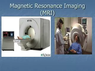
23. Tissue T1 (ms) T2 (ms) Grey Matter (GM) 950 100 White Matter (WM) 600 80 Muscle 900 50 Cerebrospinal Fluid (CSF) 4500 2200 Fat 250 60 Blood 1200 100-200 Properties of Body Tissues MRI has high contrast for different tissue types!

24. MRI of the Brain - Sagittal T1 Contrast TE = 14 ms TR = 400 ms T2 Contrast TE = 100 ms TR = 1500 ms Proton Density TE = 14 ms TR = 1500 ms

25. MRI of the Brain - Axial T1 Contrast TE = 14 ms TR = 400 ms T2 Contrast TE = 100 ms TR = 1500 ms Proton Density TE = 14 ms TR = 1500 ms

26. Brain - Sagittal Multislice T1

27. Brain - Axial Multislice T1

28. Brain Tumor T1 T2 Post-Gd T1

29. 3D Imaging • Instead of exciting a thin slice, excite a thick slab and phase encode along both ky and kz • Greater signal because more spins contribute to each acquisition • Easier to excite a uniform, thick slab than very thin slices • No gaps between slices • Motion during acquisition can be a problem

30. 2D Sequence (Gradient Echo) ky acq Gx Gy kx Gz b1 TE Scan time = NyTR TR

31. 3D Sequence (Gradient Echo) acq kz Gx Gy Gz ky kx b1 Scan time = NyNzTR

32. 3D Imaging - example • Contrast-enhanced MRA of the carotid arteries. Acquisition time ~25s. • 160x128x32 acquisition (kxkykz). • 3D volume may be reformatted in post-processing. Volume-of-interest rendering allows a feature to be isolated. • More on contrast-enhanced MRA later

33. Spectroscopy • Precession frequency depends on the chemical environment (dBcs) e.g. Hydrogen in water and hydrogen in fat have a f = fwater – ffat = 220 Hz • Single voxel spectroscopy excites a small (~cm3) volume and measures signal as f(t). Different frequencies (chemicals) can be separated using Fourier transforms • Concentrations of chemicals other than water and fat tend to be very low, so signal strength is a problem • Creatine, lactate and NAA are useful indicators of tumor types

34. Spectroscopy - Example Intensity Frequency

35. Magnetization preparation (phase and magnitude, pelc) Fast imaging (fast sequences, epi, spiral…) Motion (artifacts, compensation, correction, navigator…) MR angiography (TOF, PC, CE) Perfusion and diffusion Functional imaging (fMRI) Cardiac imaging (coronary MRA) Future lectures