Consumption
Consumption. Mankiw Chapter 16. Learning Objectives. The limitations of the Keynesian consumption function The role of interest rates in consumption The influence of age on consumption The permanent income hypothesis. The Keynesian Consumption Function.

Consumption
E N D
Presentation Transcript
Consumption Mankiw Chapter 16
Learning Objectives • The limitations of the Keynesian consumption function • The role of interest rates in consumption • The influence of age on consumption • The permanent income hypothesis
The Keynesian Consumption Function • Looking at Aggregate Demand (closed economy) • Y = C + I + G • Assuming G is exogenous, this leads to enquiring into determinants of Consumption and Investment • Consumption is of particular interest (multipliers, etc) • Previously we have: • C = (1 - s)Y (0 s < 1) • C = C(Y - T) • We need to model the behaviour of C
Keynes (1936) • Keynes (1936) made three main assertions: • C = C(Y), (not r) • 0 MPC 1, (where MPC is dC/dY) • APC falls as Y increases (APC is C/Y) • Taken together these imply a Consumption Function of the form: C = A + bY • where A and b are positive constants • APC = A/Y + b • MPC = b • and A/Y must fall as Y increases
Keynes C. Fn. As Y increases, C/Y falls: also dC/dY C/Y C 45O C = A + bY dC/dY = b A 0 Y
Empirical Evidence • Keynes hadn’t have much statistical evidence on consumption • Early estimates in the 1940s for the USA and elsewhere were conflicting. • Short-medium term annual data (1929-45) • C = A + bY; A 0; b 0.7 • Long-term data (1869-1945) • C = bY: A 0, b 0.9 • Which is “right”? • We need a proper model to answer this.
Contrasting Empirical Evidence • 1929-45: C = A + bY • 1869-45; C = b*Y C 45O b* 0.9 C = b* Y C = A + bY b 0.7 0 Y
Alternative Models • Clearly the simple Keynes approach is missing something. • We look at Three candidates • Interest rates: IntertemporalChoice model (Fisher) • Age: The Life-Cycle theory of (Modigliani, etc) • Forward looking consumers: The Permanent Income theory of Consumption (Friedman)
Intertemporal Choice • Individuals can borrow against future income to fund consumption now or save now to fund consumption in the future • Hence consumption choice is a decision on timing • Consumption will be influenced by interest rates • Specifically • Consumer chooses between consumption in different time periods • The “price” of shifting consumption between periods is the interest rate • Apply standard consumer choice theory from micro
The Micro of Consumer Choice • Budget constraint • Generally we require: PV(C) or PV(Y) • Two periods • C1 + C2 (1+r) or Y1 + Y2 (1+r) • Many Periods • Ci (1+r)i or Yi (1+r)i • Households maximize Utility over expected lifetime • U (C1, ..., Ci, ... , Cn) • Notice how this is just a special case of the standard two good model from micro
Consumer Choice Indifference Curves represent U = U(C1 , C2 ) C2 C1 0
Budget Constraint Endowment at E: OB = PV(Y) = y1 + y2 (1 + r) Slope of AB is (1 + r) Y2 A . E y2 y1 Y1 0 B
The “Price” of Consumption • Why is slope AB = - (1 + r) ? • Suppose (present) savings increase by €100 • i.e. C1 = - 100 • This allows an increase in C2 of 100(1 + r) • i.e. C2 = +100 (1 + r) • Slope AB = C2 C1 = 100 (1 + r)/ - 100 • = - (1 + r)
A Change in r An increase in r: AB pivots at E CD Y2 C A . E y2 y1 Y1 0 D B
Consumption Choice • Max U st BC • Saving is (oy1- oc*1) : future dis-saving is (oc*2 - oy2) Y2 A c*2 c* . y2 E 0 c*1 y1 B Y1
Change in Income • Y2 increases: E’ E”, AB CD, c’1 c”1 Y2 C A . E” . E’ 0 c’1 c”1 B D Y1
A Change in r when saver • Income effect 1 3; Sub effect 3 2 Y2 C F A 2 3 1 . y2 E 0 y1 Y1 c31 c21 D B G c11
Change in R when Borrower • Inc. effect 1 2; Sub. effect 2 3 Y2 C A . F E 3 1 2 0 Y1 y1 c31 c11 c21 D G B
Lessons of Intertemporal Model • Consumers are potentially forward looking • The ability to borrow or save means that consumption can be influenced by future income • Interest rates can influence consumption in potentially complicated ways • Wealth can influence consumption • All these factors were absent from the simple model
THE LIFE-CYCLE HYPOTHESIS • Income shows a marked life-cycle variation • It is low in the early years, reaches a peak in late middle age and declines, especially on retirement • Smoothing consumption over a lifetime is a rational strategy (diminishing MUy) • This implies C/Y will vary during the lifetime of an individual
THE LIFE-CYCLE HYPOTHESIS . C2 E’: low Y1/Y2 high C1/Y1 E”: high Y1/Y2 low C1/Y1 A E’ . C2* . E” C1 B 0 Y1’ C1* Y1”
THE LIFE-CYCLE HYPOTHESIS Y, C and W over the life-cycle Y, C Ct Yt Age 18 65 +W Wt Age W
THE LIFE-CYCLE MODEL • Let retirement age = 65; life expectancy = 75 • Years to retirement = R (= 65 – present age) • Expected life = T (= 75 – present age) • Assuming no pension, no discounting: • CT = W + RY is the lifetime constraint • i.e. C = (W + RY)/T • and C = (1/T)W + (R/T)Y • or C = W + Y ( = 1/T; = R/T)
THE LIFE-CYCLE MODEL • C = W + Y • MPC = C Y = • APC = C Y = (W Y) + • clearly MPC < APC • for a “typical” individual, age 35 • R=30, T = 40 • = 1/T 0.03; (MPC) = RT 0.75 • APC = [0.03 (W Y) + 0.75] > MPC
THE LIFE-CYCLE MODEL • Saving and Consumption behaviour may depend on population age-structure • Does Social Security displace personal savings? • What is the effect of Medicare (USA) or Medical Cards for over 70s (IRL) on Savings? • Savings and Uncertainty: • “rational” behaviour: run down wealth to zero • individual circumstances unpredictable (care needs) • individual life expectancy unpredictable • on average even selfish people will die with W > 0
THE PERMANENT INCOME HYPOTHESIS • Cp = kYp (0 k 1 ) • Y = Yp+ Ytr • C = Cp + Ctr • Permanent income is the return to all wealth, human and non-human: • Yp = rW • which implies: Cp = rkW • NB: C is not related to Ytr i.e. dC dYtr = 0
MEASURING PERMANENT INCOME AND CONSUMPTION (1) • Are Cpand Yp observable? • E(Ytr ) = 0 • E(Ctr ) = 0 • which imply that E(Y) = E(Yp ), etc. • However this is ex ante: ex post, actual measures may reveal more • (a) in a recession: Y < Yp : Ytr < 0 • (b) in a boom: Y > Yp : Ytr > 0
MEASURING PERMANENT INCOME AND CONSUMPTION (2) • Cross-section measurements of C and Y C 45o Ci, Yi. . . . . Ci = A + bYi . . Cm . 0 Y Ym
MEASURING PERMANENT INCOME AND CONSUMPTION (3) • Where Yj > Ym, Ytr > 0 and Yj > Ypj C 45o Cp =kYp Cj Ci = A + bYi Cm Ytrj 0 Y Yj Ym Ypj
MEASURING PERMANENT INCOME AND CONSUMPTION (4) • Aggregate: Ytr > 0 in boom, < 0 in recession • Measured C/Y should be < in boom than in recession (Recent experience?) • Aggregate Ctr = 0: individual Ctr is > or < 0 • Average Ctr = 0 for all income groups • Measuring Yp: • Adaptive expectations: Yp = f(Yt, Y t - 1, ...Y t-n) • Rational expectations: only new information (shocks) change Yp • Consumption V Consumption Expenditure, which highlights the role of durables (Investment and saving rather than consumption
MEASURING PERMANENT INCOME AND CONSUMPTION (5) • Also we may express the PYH as an error-correction model: • Ypt = Ypt-1 + j(Yt – Ypt-1) 0 < j < 1 • which with: Ct = Cpt = kYpt • gives: Ct = kYpt = kYpt-1 + kj(Yt – Ypt-1) • Re-arranging: Ct = (k – kj)Ypt-1 + kjYt • j 0 implies slow adaptation, j 1 implies rapid adaptation • assume k = 0.9, j = 0.3, so kj = 0.27 • then: Ct = (0.9 – 0.27)Ypt-1 + 0.27Yt or 0.63Ypt-1 + 0.27Yt • However this is not an explicitly forward-looking model. • Now suppose C = Cp = kYp, then Yp = 1/k(Cp) • Thus Ct = (0.63/k)Ct – 1 + 0.27Yt = 0.7Ct – 1 + 0.27Yt
PERMANENT INCOME AND RECESSION • Y < Yp in short-run (mild) recession • Suppose there is a shock to the system (financial crisis) • Pwople expect a severe long-drawn-out recession: i.e. Yp falls, ie. E(Y) falls • It is possible that initiallyY > Yp • C (and Cp) will fall • If people anticipate a fall in Yp, then C/Y may fall • Current (mid-2009) situation: big fall in W, both the Permanent and Life-cycle theories predict that this will hit C (independently of current measured Y)