Fitting Non-Linear Regression Models V&R 8.2
Fitting Non-Linear Regression Models V&R 8.2. Oy Mae Louie Bessie Nguyen Gina Piscitelli. When do we use a non-linear regression model? . When at least one of the parameters is not linear The general form of a non-linear regression model is y= η (x, β ) + ε where ε ~N(0, σ 2 ).

Fitting Non-Linear Regression Models V&R 8.2
E N D
Presentation Transcript
Fitting Non-Linear Regression Models V&R 8.2 Oy Mae Louie Bessie Nguyen Gina Piscitelli
When do we use a non-linear regression model? • When at least one of the parameters is not linear • The general form of a non-linear regression model is y=η(x,β) + ε where ε ~N(0, σ2)
oldpar<-par(mar=c(5.1,4.1,4.1,4.1)) plot(Days,Weight,type="p",ylab="Weight(kg)") Wt.lbs<-pretty(range(Weight*2.2025)) axis(side=4,at=Wt.lbs/2.205,lab=Wt.lbs,srt=90) mtext("Weight(lb)",side=4,line=3) Plot of Weight Loss vs Days for an Obese Patient
Model: y = βo + β1*2-t/θ + ε The parameters: βo: ultimate lean weight β1: total amount of weight to be lost θ: time taken to lose half the amount of weight remaining to be lost Weight Loss Dataset
Method Used to Analyze Data • Iterative procedure • The number of iterations depend on how quickly the parameters converge. • The converged parameters are close approximates for βo,β1,and θ. • The likelihood for the non-linear regression model is maximized when residual sum of squares is minimized.
Non-Linear Regression Methods 1. "Direct Computation" Method: y = βo + β1*2-t/θ • "Derivative" Method: η(β) ≈ ω(0) + Z(0)β • Self-Starting Method: y = βo + β1 exp(-x/θ) + ε
1. Direct Computation Method The direct computation method initializes values for b0, b1, and theta by inspection of the weight loss data set. R Code wtloss.st <-c(b0 = 90, b1 = 95, th =120) wtloss.fm <- nls(Weight ~ b0 + b1*2^(-Days/th), data = wtloss, start = wtloss.st, trace = T) wtloss.fm lines(Days,fitted.values(wtloss.fm))
2. Derivative Method • The equation η(β) ≈ ω(0) + Z(0)β defines (in vector terms) the tangent plane to the surface at the coordinate point β = β(0) where • η(β) is the mean vector • ω(0)is the offset vector • Z (0) is the matrix which defines the tangent plane • Each iteration gives a new approximation for βuntil convergence is reached. • The derivative method uses numerical methods to compute a formula for the gradient unless first derivatives are supplied.
2. Derivative Method (continued) • The symbolic differentiation function deriv can be used to automatically generate the desired function. R code expn1<-deriv (y ~ b0 + b1 * 2 ^ (-x/th),c('b0','b1','th'), function(b0,b1,th,x){}) wtloss.gr <-nls(Weight ~expn(b0, b1, th, Days), data = wtloss, start = wtloss.st, trace = T) lines(Days,fitted.values(wtloss.gr))
3. Self-Starting Method The self starting method fits a non-linear model without explicit initial values. Procedure a) Fit Quadratic Regression b) Find fitted values y0, y1, and y2 and three equally spaced points x0, x1 = x0 + δ and x2 = x0 + 2δ c) Find initial value of θ using the following formula: θo = δ / log ((y0 – y1)/(y1-y2)) d) Find initial values for β0 and β1 by obtaining linear regression of y on exp(-x/ θo)
3. Self-Starting Method (continued) R code negexp<-selfStart(model = ~b0 + b1*exp(-x/th), initial = negexp.SSival,parameters=c("b0","b1","th"), template=function(x,b0,b1,th){}) wtloss.ss<-nls(Weight~negexp(Days,B0,B1,theta), data=wtloss,trace=T) lines(Days,fitted.values(wtloss.ss))
Direct Computation Method SSR B0 B1 theta 67.54349 : 90 95 120 40.18081 : 82.72629 101.30457 138.71374 39.24489 : 81.39868 102.65836 141.85859 39.2447 : 81.37375 102.68417 141.91052 Derivative Method SSR B0 B1 theta 67.54349 : 90 95 120 40.18081 : 82.72629 101.30457 138.71374 39.24489 : 81.39868 102.65836 141.85859 39.2447 : 81.37375 102.68417 141.91053 Self Starting Method SSR B0 B1 theta 82.71307 101.49465 200.16004 39.54532 : 82.71307 101.49465 200.16004 39.245 : 81.39823 102.65882 204.65214 39.2447 : 81.37374 102.68418 204.73363 B0 and B1: For all three methods, the approximated values for B0 and B1 are about the same. Theta: For both the direct computation and derivative method, the approximated values for theta are about the same. However, for the self starting method, the theta is different. For the Weight Loss data, three iterations are necessary for the values of B0, B1 and theta to converge. Results
Results • Model: Weight ~ β0 + β1 * 2-Days/θ • β0 = 81.37375 • β1= 102.68417 • θ = 141.91052 • residual sum-of-squares: 39.2447 • Model: y = 81.374 + 102.68 * 2-Days/141.91
Summary • Use a non-linear regression model when at least one of the parameters is not linear. • Non-linear regression is an iterative procedure in which the number of iterations depend on how quickly the parameters converge. • Three methods introduced: • Direct Computation Method • Derivative Method • Self-Starting Method