Download
1 / 28
280 likes | 527 Vues
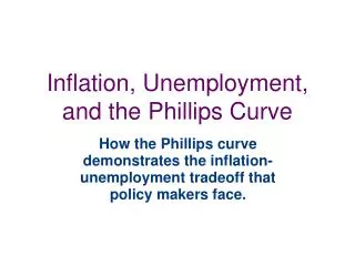
Inflation, Deflation, and the Phillips Curve. Inflation Deflation. Macroeconomics up to now. i. r. IS-MP. Y. u. Y pot. Potential output = AF(K,L). Now add inflation. i. r. IS-MP. Y. π e. u. Y pot.

E N D
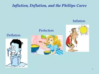
Inflation, Deflation, and the Phillips Curve Inflation Deflation
Macroeconomics up to now i r IS-MP Y u Ypot Potential output = AF(K,L)
Now add inflation i r IS-MP Y πe u Ypot Potential output = AF(K,L) π
How do we measure price indexes? Consumer price index: • Traditionally a Laspeyres price index (fixed weight index using early prices) • BLS has introduced an experimental index – the “chain CPI” – which is a superlative Törnqvist index. • As with output index, Laspeyres overstates inflation: g(Paasche) < g(Tornqvist), g(Fisher) < g(Laspeyres) National accounts price indexes • These are Fisher (superlative) indexes • Fed target uses personal consumption expenditures price index (Fisher) “Core Inflation” - removes volatile food and energy and is central target for monetary policy (personal consumption core price index)
Laspeyres Superlative: Fisher, Tornqvist Paasche
Does it make any difference?Yes, 0.5% per year over 1970-2012
Major topics • Why do we care about inflation? • Modern inflation theory
Why do we care about inflation? Like temperature, we care mainly about the extremes: Hyperinflation (> 100% a month) Deflation (< 0)
What are costs of inflation? • Redistribution: inflation redistributes wealth from creditors to debtors (mortgages, pensions). • Inefficiencies of inflation: shoe leather, menu costs, taxes,... • Distinguish anticipated from unanticipated inflation (ex ante v. ex post real interest rates) • Overall, costs appear relatively small at low inflation rates. • Hyperinflation can destroy price mechanism • Deflation can produce low-level equilibrium
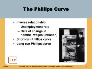
The Expectations -Augmented Phillips Curve Fundamentals of theory: • Unemployment rate (u) determined by interaction of potential and actual Y by Okun’s Law • Inflation determined by labor/product market tightness (u relative to “natural rate of unemployment”*) and expected inflation (πe) – Phillips curve • Expected inflation (πe) determined by inflation history and forecasts of future inflation *natural rate of unemployment (Jones); sometimes called the NAIRU = “non-accelerating inflation rate of unemployment” = Goldilocks unemployment rate
The Expectations -Augmented Phillips Curve In algebra: u - u* = λ (Y – YP)/YP π= πe - β (u - u*) πe determined by past inflation and expectations process
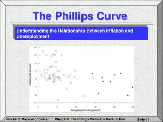
The short-run P.C. Graph from Economic Report of the President 1969 This was relationship that led Keynesian to believe that P.C. was a good explanation for inflation (1960s) • (πe)
Collapse of short-run P.C. This was relationship that led many new classical economists to conclude that Keynesian theories were “fatally flawed” (Lucas and Sargent. 1970s)
Mainstream 2-equation inflation model • π(t) = πe(t) + β[u(t) - u*] + ε(t) • πe(t) = π(t-1) Endogenous variablesπ = rate of price inflationπe = expected rate of inflation (or similar concept)u* = natural rate Exogenous variablesu = actual unemployment rate (determined by policy and shocks)ε(t) = wage and price shocks (oil prices, exchange rates, globalization, decline of unions, immigration, etc...)t = time [Note: (2) is backward looking rather than rational expectations.]
Simplest 1-equation inflation model Simplify by assuming no shocks and substituting: (3) π(t) = π(t-1) - β[u(t) - u*] • Δ π(t) = - β[u(t) - u*] which is the linear expectations-augmented P.C. model.
Short-run Phillips curve π1 = π1e 1 SRPC1 u* = natural rate
Moving up short-run Phillips curve π2 2 π1 = π1e 1 SRPC1,2 u* = natural rate
Short-run Phillips curve shifts upward with higher inflation expectations π3e=π2 2 π1 = π1e 1 SRPC3 SRPC1,2 u* = natural rate
Now unemployment rate back to the natural rate 3 π3= π3e 2 π1 = π1e 1 SRPC3 SRPC1,2 u* = natural rate
u equals the natural rate in both periods 1 and 3, but the expected and actual inflation rates are higher in period 3. This diagram shows the way that the SRPC shifts as expected inflation adjusts to higher rate. LRPC 3 π3e=π2 2 π1 = π1e 1 SRPC3 SRPC1,2 u* = natural rate
New synthesis of accelerationist PC Rough estimate of natural rate for 1960-2012 = 6 percent Δ π(t) = β[u(t) - u*] u* is u where Δ π(t) =0. This was the new synthesis developed by Phelps and Friedman (1967-68). It now forms the basis of mainstream macro for large open economies. 25 25
Phillips curve at low inflation Does Phillips curve bend because of nominal rigidity at zero inflation? Controversial, but probably yes. 1-2% u* = natural rate 26
Summary onThe Expectations-Augmented Phillips Curve • u and π are negatively related in short run • no relation between u and π in the long run • short-run PC adjusts up and down as economic agents adjust their inflation expectations to reality (combination of backward and forward looking expectations). • Natural rate is u at which inflation tends neither to rise nor fall
Deflation Deflation = falling price level This seldom occurs in modern economy, but sometimes have near-zero inflation (Japan for two decades, US today). Problems: - If full-employment interest rate < 0, have liquidity trap - Unstable dynamics: since r = i – π, asπfalls have higher real interest rate, lower I, lower Y, and “low-level trap” Some of the issues involved are discussed in Bullard, Seven Faces. Very interesting discussion! But this is uncharted territory in modern macro!