

SlideServe
Menu
Préférences
© SlideServe · v2026

The Phillips Curve

bree avatar
19 diapositives · 474 Views · Jan 23, 2013

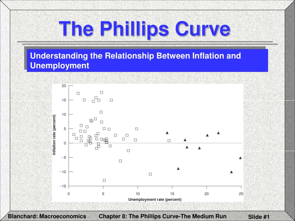
The Phillips Curve. Understanding the Relationship Between Inflation and Unemployment. The Phillips Curve-Understanding the Relationship Between Inflation and Unemployment. An inverse relationship between inflation and unemployment until the 1970s 1970s high inflation and unemployment
The Phillips Curve - slide 1
01 / 19The Phillips Curve
1 / 17

Télécharger la présentation

The Phillips Curve
Une image / un lien ci-dessous est fourni (tel quel) pour télécharger la présentation

Politique de téléchargement : le contenu du site vous est fourni TEL QUEL pour votre information et votre usage personnel ; il ne peut être vendu, concédé sous licence ni partagé sur d’autres sites sans l’accord de son auteur.Le contenu vous est fourni TEL QUEL, pour votre information et votre usage personnel uniquement. Téléchargez la présentation en cliquant sur ce lien. Lors du téléchargement, si vous ne parvenez pas à télécharger une présentation, l’éditeur a peut-être supprimé le fichier de son serveur.Pendant le téléchargement, si vous ne parvenez pas à obtenir une présentation, le fichier a peut-être été supprimé par l’éditeur.

F I N

Plus de contenu associé

Transcription de la présentation
  1. The Phillips Curve Understanding the Relationship Between Inflation and Unemployment

  2. The Phillips Curve-Understanding the Relationship Between Inflation and Unemployment • An inverse relationship between inflation and unemployment until the 1970s • 1970s high inflation and unemployment • Is there still a relationship between inflation and unemployment?

  3. The Phillips Curve – Understanding Inflation, Expected Inflation, and Unemployment From our wage setting – price setting model: Wt = PteF(ut,z) and Pt = (1+µ) Wt Lets assume that F(ut,z) = 1-ut+z Then Pt = Pte(1+µ)F(ut,z) Pt = Pte(1+µ) (1-ut+z)

  4. The Phillips Curve – Understanding Inflation, Expected Inflation, and Unemployment From Pt = Pte(1+µ) (1-ut+z) We can derive t =  t e + (µ+z)-ut where t = the inflation rate  t e = the expected inflation rate

  5. The Phillips Curve – Understanding Inflation, Expected Inflation, and Unemployment Observations:  t =  t e + (µ+z) - ut • Higher expected inflation leads to higher inflation • Given expected inflation, the higher the µ or z, the higher inflation • Given expected inflation, the higher unemployment, the lower inflation

  6. The Phillips Curve – Understanding Inflation, Expected Inflation, and Unemployment The Early Incarnation, Circa 1960 • Average inflation close to zero •  t e = O •  t = (µ+z) - ut • Low unemployment leads to high wage increases leads to high price increases leads to high wage increases in a wage – price spiral.

  7. The Phillips Curve – Understanding Inflation, Expected Inflation, and Unemployment The Early Incarnation, Circa 1960

  8. 1970s: Why did the Phillips curve vanish?higher oil prices increased µandinflation became persistent andpositive

  9. The Phillips Curve – Understanding Inflation, Expected Inflation, and Unemployment Inflation & Expectations

  10. Assume: The Phillips Curve – Understanding Inflation, Expected Inflation, and Unemployment Inflation & Expectations • the effect of last year’s inflation rate on this year’s expected inflation rate • the higher the value of , the higher the expected inflation rate

  11. The Phillips Curve – Understanding Inflation, Expected Inflation, and Unemployment Mutations & Expectations • 1900-1960: Inflation low and not persistent •  = 0, te =  t-1 = 0 and • t= (µ+z) – ut (the normal Phillips Curve)

  12. The Phillips Curve – Understanding Inflation, Expected Inflation, and Unemployment Mutations & Expectations • 1970s: Inflation high and persistent •  started to increase to 1 • t=  t-1 + (µ+z) – ut ( t-1 = te ) • The inflation rate depends on: • The unemployment rate (ut) • Last year’s inflation rate ( t-1)

  13. The Phillips Curve – Understanding Inflation, Expected Inflation, and Unemployment Inflation & Expectations When: t=  t-1 + (µ+z) – ut and = 1 Aggregate supply = t – t-1 = (µ+z) – ut Therefore: The unemployment rate affects the change in the inflation rate High unemployment decreases inflation the inflation rate

  14. Inflation & Expectations 1970-1998: t – t-1 = 6.5% – 1.0ut

  15. The Phillips Curve – Back to the Natural Rateof Unemployment At the natural rate of unemployment (un): The actual inflation rate = expected inflation ratet = te • Given: t – te + (µ+z) – un • Then: 0 = (µ+z) – un

  16. Given: The Nonaccelerating Inflation Rate of Unemployment (NAIRU) Then: un = µ + z Given: t = te + (µ+z) – ut Then: t = te + un – ut t – te = -(ut – un) ut – un  t =te

  17. The Phillips Curve – A Summary and Many Warnings Summary: The AS relation: t – t-1 = -(ut – un) shows that: Inflation increases when ut > un Inflation decreases when ut < unHowever: the relation can shift

  18. m + µ and z are assumed consistent t = u n L The Phillips Curve – Differences in the Natural Rate Across Countries • Changes in u and z • The composition of the labor force • The structure of wage bargaining • Unemployment benefits • Can you think of others?

  19. The Phillips Curve – Differences in the Natural Rate Across Countries The Limits of Our Understanding Europe in the 1990s