Download
1 / 13
130 likes | 194 Vues
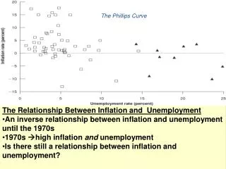
Investigate the Phillips Curve and inflation behavior, role of price and inflation expectations, with a focus on AS theory. Learn about US unemployment trends, tradeoffs, and implications for policy decisions.

E N D
Aggregate Supply and the Phillips Curve Chapter #6
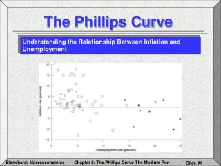
Inflation and Unemployment • To further develop AS side of the econ (dynamic adjustment from short to long run) examine P-Y relationship based on links between wages, P, employment & Y. • Introduce role of price & inflation expectations & “rational expectations revolution” • AS theory is the least settled area in macro • Don’t fully understand why W and P are slow to adjust, but offer several theories • All differ in starting point, but reach same conclusion: flat SRAS & vertical LRAS • U.S. unemployment over several decades • High unemployment: early 1960s, mid 1970’s, early-mid 1980’s, early 1990s & current • Low unemployment: late 1960’s, early 2000 & 2007 • Phillips curve (PC) shows unemployment & inflationrelationship (translate Y into unemployment & P into inflation) • Although Y is linked to unemployment, easier to work with PC than AS when discussing unemployment
The Phillips Curve • In 1958 Phillips published a study of wagebehavior in UK between 1861 & 1957 • The main findings are: Unemployment % & wage inflation inversely related Policy: Unemployment % & wage inflation tradeoff • Unemployment ↓ wage inflation gw = Wt+1/Wt- 1. • Simple PC is defined as: gw = -(u - u*),where u* is natural rate of unemployment, is wages responsiveness to unemployment,& (u - u*) is unemployment gap. • Wages are falling when u > u*. • Given econ in equilibrium (stable prices & unemployment at the natural rate),if money supply ↑ 10% wages & prices must ↑ 10% for econ to return to equilibrium • PC: wages ↑ => unemployment ↓, price ↑ & econ returns to full employment level • To see why this is so, rewrite PC in terms of wage levels: gw = Wt+1/Wt- 1 = -(u - u*) => Wt+1 = Wt [1 - (u - u*)]For wages to rise above previous levels, u must fall below the natural rate
The Policy Tradeoff • PC became a cornerstone of macro policy analysis since it suggests that policy makers could choose combinations of u and rates Choose low u if willing to accept high (late 1960’s) Maintain low by having high u (early 1960’s) • In reality u & short run tradeoff Tradeoff disappears as AS becomes vertical • & u behavior in US since 1960 does not fit simple PC story Individuals concerned with standard of living & compare wage growth to inflation. If wages do not “keep up” with inflation, standard of living falls Individuals form e over a particular period of time & use in wage negotiations • Rewrite PC to reflect this: gw - e = - (u - u*) • If maintaining assumption of a constant real wage (W/P) actual = gwwage inflation, • Modern or the expectations augmented PC is: - e = - (u - u*) => = e - (u - u*) NOTE: 1. e passes one for one into actual 2. u = u* when e =
Inflation Expectations-Augmented PC • Modern PC intersects natural rate of unemployment at level of expected inflation • Inflation expectations-augmented PC for the 1980s and early 2000 • The height of the SRPC depends upon e • Changes in expectations shifts PC ↑ & ↓ • e adds another automatic adjustment mechanism to AS side of the economy • When high AD moves the economy up and to the left along the SRPC causing • if persists, people adjust their expectations upwards, and move to higher SRPC • How does the augmented PC hold up? • To test augmented PC need to measure e best estimate is last period’s , e = t-1 • Augmented PC using the equation: - e ≈ - t-1 = - (u – u*) Appears to work well in most periods
Rational Expectations • The augmented PC predicts: actual rises above e when u < u* So why don’t individuals quickly adjust their expectations? • The PC relies on people being WRONG about in a very predictable way • If people learn to use (4) to predict , e should always equal , and thus u = u* • Robert Lucas modified the model to allow for mistakes • Good econ model should not rely on public making easily avoidable mistakes • So long as our predictions are based on information available to public, the values we use for e should be the same as the values the model predicts for • Surprise shifts in AD will change unemployment, but predictable shifts will not • The argument over rational expectations is as follows: • Usual macro model takes PC height as being pegged in the SR by e, where e is set by historical experience • The rational expectations model has the SRPC floating up and down in response to available information about the near future • Individuals use new information to update their expectations • Both models agree that if money growth were permanently increased, the PC would shift up in the LR, and would increase with no LR change in u • The RE model states that this change is instantaneous, while the traditional model argues that the shift is gradual
Wage-Unemployment Relationship & Sticky Wages • Neoclassical (vertical) AS: wages adjust instantly to ensure full employment Y*. BUT Y is not always at Y*. PC: wages adjust slowly to changes in unemployment • The key question in AS theory: “Why are wages sticky?” or Why does nominal wage adjust slowly to shifts in demand, allowing for econ to deviate from Y*? • To clarify sticky wages translate (u - u*) into employment levels. If labor force is 100 => u* = 5% N* (Y*) = 95 & u = 7% N (actual employment) = 93.u - u* = (N* - N)/N* = 1 - N/N*, numerically 0.07 - 0.05 = 1 - 93/95 = 0.02. • Using gw = Wt+1/Wt- 1, modern PC: gw - e = - (u - u*) & unemployment gap in employment levels, we get: gw - e = Wt+1/Wt- 1 - e = - (1 - N/N*) or Wt+1 = Wt[1 + e - (1 - N/N*)] • Next period equals this period wage with adjustment for employment level & e • At full employment N* = N, this period wage equals last period wage plus adjustment for e • If N > N*, this period wage exceeds last period’s by more than e since- (1 - N/N*) > 0 or gw - e > 0.
Wage-Unemployment Relationship & Sticky Wages • Figure illustrates the wage-employment relationship, WN • The extent to which the wage responds to E depends on the parameter • If is large, u has large effects on wages and the WN line is steep • The PC relationship also implies WN relationship shifts over time • If there is over-employment this period, WN shifts up to WN’ • If there is less than full employment this period, WN curve shifts down to WN’’ Result: AD changes altering u this period will have effects on wages in subsequent periods
Wage-Unemployment Relationship & Sticky Wages • Each school of thought has to explain PC existence, or why wage & price are sticky • Examples of such explanations for wage and price stickiness include: • Imperfect information (workers wrongly interpret inflation as real wage ↑ => work more) • In the context of clearing markets • Coordination problems (lack of in market => firms slowly ↑ not to loose demand) • Focus on the process by which firms adjust their prices when demand changes • Efficiency wages &costs of price changes (pay above market W to keep & motivate N) • Focus on wage as a means of motivating labor • Explanation of wage stickiness builds on these theories and one central element the labor market involves long-term relationships between firms and workers • Work conditions, including wage, renegotiated periodically & infrequently, due to the costs • At any time, firms and workers agree on a wage schedule to be paid to currently employed workers • If demand for labor increases and firms increase hours of work, in the SR wages rise along the WN curve • With demand up, workers press for increased wages, but takes time to renegotiate all wages (staggered wage-setting dates) • During the adjustment process, firms also resetting P to cover increased cost of production • Process of W and P adjustment continues until economy back at full employment level of output
Transition From PC to AS Curve in 4 Steps • 1. Translate output to employment: Close short run unemployment output relationship. • Okun’s Law: Y/Y* - 1 = -(u - u*). Estimate ≈ 2 1% of unemployment costs 2% of Y • 2. Link prices firms charge to costs: Firms charge price that at least ≥ costs of production • Assuming N is the only cost of production, if each unit of N produces a units of output, • costs of production per output is W/a. P set as markup on labor cost, z: P = (1+z)W/a. • 3. Use PC wage/employment relationship: Note that price inflation = wage inflation • = Pt+1/Pt -1 = [aWt+1/(1+z)]/[aWt/(1+z)] - 1 = Wt+1/Wt-1 = gw • Substitute for gw in gw - e= - (1 - N/N*) => - e=- (1 - N/N*) = - (u - u*). • Combined with (Y/Y* - 1)/= -(u - u*) from Okun’s Law: - e=(/)(Y/Y* - 1). • 4. Derive upward sloping AS curve combining 1-3: • Use ≡: (Pt+1/Pt - 1) – (Pt+1e/Pt - 1) = (Pt+1 - Pt+1e)/Pt (Pt+1 - Pt+1e)/Pt=(/)(Y/Y* - 1), solve for Pt+1 • Pt+1= Pt+1e + Pt(/)(Y/Y* - 1) • AS curve: Pt+1≈ Pt+1e[1 + λ(Y - Y*)] • If Y > Y*, next period AS curve shifts left to AS’ • If Y < Y*, next period AS curve shifts right to AS’’ • NOTE: These are the same properties as the WN curve
Supply Shocks • A supply shock is an econ disturbance whose first impact is a shift in the AS curve • An adverse supply shock shifts AS inwards • As AS shifts to AS’, equilibrium shifts from E to E’ and prices increase while output falls • The unemployment at E’ forces wages & prices down until return to E, but process is slow • After the shock: • Economy returns to full employment level • Price level is the same as it was before the shock • Nominal wages are LOWER due to the increased unemployment at the onset of the shock • Real wages must also fall where w is the real wage and W is the nominal wage • Impact of AD policy after an adverse supply shock • Suppose G increases (to AD’): • Economy could move to E* if increase enough • Such shifts = “accommodating policies” (accommodate the fall in the real wage at the existing nominal wage) • Added inflation, although reduce u from AS shock
Evaluating u & Tradeoff • Gallup organization conducts opinion polls: “What is the most important problem facing the country?” • Unemployment become the most important one • What are the relative economic costs of inflation and unemployment? • The greatest cost = lost production • This cost is large: a recession can easily cost 3-5% of GDP and hundreds of billions of dollars • Okun’s law states that 1 extra point of unemployment costs 2% of GDP • Costs borne unevenly, largely by those who lose their jobs • Workers just entering the labor force and teenagers are amongst the hardest hit
Studies interactions between economic policy decisions and political considerations Building blocks: 1. What are the tradeoffs from which a policymaker can choose? 2. How do voters rate the issues? 3. What is the optimal timing for influencing election results? Voters worry about level&rate of change of unemployment & inflation, especially 1. Rising unemployment 2. Inflation that differs from expectations These worries influence types of policies used Policymaker wants economy pointing in the right direction at election time How to use time between inauguration & election to bring econ to the right position? 1. Use restrictive policies early to raise unemployment and lower inflation 2. As election approaches, use expansionary policy to lower unemployment Should be a systematic cycle in unemployment, which is not observed in real life Factors against PBCT:1. Ability of government to fine tune the economy is limited 2. Difficulties of implementing politically motivated manipulations - Midterm elections - Risks of cynical manipulation of macroeconomic policies - Macroshocks overshadowing election cycle - Executive branch does not control full range of instruments (independ Fed) - Rational expectations Political Business Cycle Theory