SIMC Tuning Rules for Step Response Analysis Quiz
280 likes | 372 Vues
Learn to suggest PI-tunings using the SAC method for different time constants, understand plant approximation, factors impacting control, and the cascade control method. Gain insights into obtaining and interpreting the model from step responses.

SIMC Tuning Rules for Step Response Analysis Quiz
E N D
Presentation Transcript
SIMC-tunings QUIZ Quiz: SIMC PI-tunings y y Step response t [s] Time t (a) The Figure shows the response (y) from a test where we made a step change in the input (Δu = 0.1) at t=0. Suggest PI-tunings for (1) τc=2,. (2) τc=10. (b) Do the same, given that the actual plant is
QUIZ Solution • Actual plant:
QUIZ Approximation of step response Approximation ”bye eye”
SIMC-tunings Kc=2.9, tauI=10 Kc=9.5, tauI=10 OUTPUT y INPUT u • Tunings from Step response “by eye” model • Setpoint change at t=0, input disturbance = 0.1 at t=50 Tunings from Half rule (Somewhat better) Kc=2, tauI=5.5 Kc=6, tauI=5.5
QUIZ Half-rule approach: Approximation of zeros depends on tauc!
Some discussion points • Selection of τc: some other issues • Obtaining the model from step responses: How long should we run the experiment? • Cascade control: Tuning • Controllability implications of tuning rules
Selection of c: Other issues • Input saturation. • Problem. Input may “overshoot” if we “speedup” the response too much (here “speedup” = /c). • Solution: To avoid input saturation, we must obey max “speedup”:
A little more on obtaining the model from step response experiments 1¼ 200 (may be neglected for c < 40) • “Factor 5 rule”: Only dynamics within a factor 5 from “control time scale” (c) are important • Integrating process (1 = 1) Time constant 1 is not important if it is much larger than the desired response time c. More precisely, may use 1 =1 for 1 > 5 c • Delay-free process (=0) Delay is not important if it is much smaller than the desired response time c. More precisely, may use ¼ 0 for < c/5 time ¼ 1 (may be neglected for c > 5) c = desired response time
Step response experiment: How long do we need to wait? • RULE: May stop at about 10 times effective delay • FAST TUNING DESIRED (“tight control”, c = ): • NORMALLY NO NEED TO RUN THE STEP EXPERIMENT FOR LONGER THAN ABOUT 10 TIMES THE EFFECTIVE DELAY () • EXCEPTION: LET IT RUN A LITTLE LONGER IF YOU SEE THAT IT IS ALMOST SETTLING (TO GET 1 RIGHT) • SIMC RULE: I = min (1, 4(c+)) with c = for tight control • SLOW TUNING DESIRED (“smooth control”, c > ): • HERE YOU MAY WANT TO WAIT LONGER TO GET 1 RIGHT BECAUSE IT MAY AFFECT THE INTEGRAL TIME • BUT THEN ON THE OTHER HAND, GETTING THE RIGHT INTEGRAL TIME IS NOT ESSENTIAL FOR SLOW TUNING • SO ALSO HERE YOU MAY STOP AT 10 TIMES THE EFFECTIVE DELAY ()
“Integrating process” (c < 0.2 1): Need only two parameters: k’ and From step response: Example. Step change in u: u = 0.1 Initial value for y: y(0) = 2.19 Observed delay: = 2.5 min At T=10 min: y(T)=2.62 Initial slope: Response on stage 70 to step in L y(t) 2.62-2.19 7.5 min =2.5 t [min]
Example (from quiz) Step response Δu=0.1 • Assume integrating process, theta=1.5; k’ = 0.03/(0.1*11.5)=0.026 • SIMC-tunings tauc=2: Kc=11, tauI=14 (OK) • SIMC-tunings tauc=10: Kc=3.3, tauI = 46 (too long because process is not actually integrating on this time scale!) INPUT y OUTPUT y tauc=10 tauc=2
Cascade control Cascade control
Cascade control Tuning of cascade controllers • Want to control y (primary CV), but have “extra” measurement y 1 2 • Idea: Secondary variable (y ) may be tightly controlled and this 2 helps control of y . 1 • Implemented using cascade control: Input (MV) of “primary” controller (1) is setpoint (SP) for “secondary” controller (2) • Tuning simple: Start with inner secondary loops (fast) and move upwards • Must usually identify ”new” model ( G1’ = G1 G21 K2 (I+K2G22)-1 ) experimentally after closing each loop • One exception: Serial process, G21 = G22 2 – Inner (secondary - 2) loop may be modelled with gain=1 and effective delay=( t + q ) c 2 See next slide
Cascade control Special case: Serial cascade y2 = T2 r2 + S2d2, T2 = G2K2(I+G2K2)-1 • K2 is designed based on G2 (which has effective delay 2) • then y2 = T2 r2 + S2 d2 where S2¼ 0 and T2¼1 · e-(2+c2)s • T2: gain = 1 and effective delay = 2+c2 • NOTE: If delay is in meas. of y2 (and not in G2) then T2¼ 1 ·e-c2s • SIMC-rule: c2 ≥ 2 • Time scale separation: c2≤c1/5 (approximately) • K1 is designed based on G1’ = G1T2 • same as G1 but with an additional delay 2+c2
Cascade control ys y2 y2s u G2 G1 K1 K2 y1 Example: Cascade control serial process d=6 Use SIMC-rules! Without cascade With cascade
Cascade control Tuning cascade control
Cascade control Tuning cascade control: serial process • Inner fast (secondary) loop: • P or PI-control • Local disturbance rejection • Much smaller effective delay (0.2 s) • Outer slower primary loop: • Reduced effective delay (2 s instead of 6 s) • Time scale separation • Inner loop can be modelled as gain=1 + 2*effective delay (0.4s) • Very effective for control of large-scale systems
Setpoint overshoot method Alternative closed-loop approach:Setpoint overshoot method • Procedure: • Switch to P-only mode and make setpoint change • Adjust controller gain to get overshoot about 0.30 (30%) • Record “key parameters”: • 1. Controller gain Kc0 • 2. Overshoot = (Δyp-Δy∞)/Δy∞ • 3. Time to reach peak (overshoot), tp • 4. Steady state change, b = Δy∞/Δys. • Estimate of Δy∞ without waiting to settle: Δy∞ = 0.45(Δyp + Δyu) • Advantages compared to Ziegler-Nichols: • * Not at limit to instability • * Works on a simple second-order process. Closed-loop step setpoint response with P-only control. M. Shamsuzzoha and S. Skogestad, ``The setpoint overshoot method: A simple and fast method for closed-loop PID tuning'', Journal of Process Control, 20, xxx-xxx (2010)
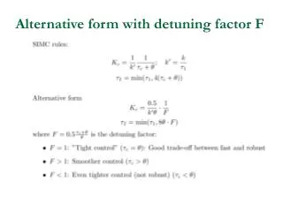
Proposed PI settings (including detuning factor F) Setpoint overshoot method Summary setpoint overshoot method From P-control setpoint experiment record “key parameters”: 1. Controller gain Kc0 2. Overshoot = (Δyp-Δy∞)/Δy∞ 3. Time to reach peak (overshoot), tp 4. Steady state change, b = Δy∞/Δys Choice of detuning factor F: • F=1. Good tradeoff between “fast and robust” (SIMC with τc=θ) • F>1: Smoother control with more robustness • F<1 to speed up the closed-loop response.
Setpoint overshoot method Example: High-order process P-setpoint experiments Closed-loop PI response
Setpoint overshoot method Example: Unstable plant First-order unstable process • No SIMC settings available Closed-loop PI response
CONTROLLABILITY A comment on Controllability • (Input-Output) “Controllability” is the ability to achieve acceptable control performance (with any controller) • “Controllability” is a property of the process itself • Analyze controllability by looking at model G(s) • What limits controllability?
CONTROLLABILITY Controllability Recall SIMC tuning rules 1. Tight control: Select c= corresponding to 2. Smooth control. Select Kc ¸ Must require Kc,max > Kc.min for controllability ) max. output deviation initial effect of “input” disturbance y reaches k’ ¢ |d0|¢ t after time t y reaches ymax after t= |ymax|/ k’ ¢ |d0|
CONTROLLABILITY Controllability
CONTROLLABILITY Example: Distillation column
CONTROLLABILITY Example: Distillation column
CONTROLLABILITY Conclusion controllability • If the plant is not controllable then improved tuning will not help • Alternatives • Change the process design to make it more controllable • Better “self-regulation” with respect to disturbances, e.g. insulate your house to make y=Tin less sensitive to d=Tout. • Give up some of your performance requirements