Download
1 / 12
120 likes | 275 Vues
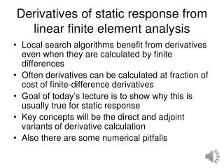
Derivatives of static response from linear finite element analysis. Local search algorithms benefit from derivatives even when they are calculated by finite differences Often derivatives can be calculated at fraction of cost of finite-difference derivatives

E N D
Derivatives of static response from linear finite element analysis • Local search algorithms benefit from derivatives even when they are calculated by finite differences • Often derivatives can be calculated at fraction of cost of finite-difference derivatives • Goal of today’s lecture is to show why this is usually true for static response • Key concepts will be the direct and adjoint variants of derivative calculation • Also there are some numerical pitfalls
Properties of governing equations • Equations of equilibrium in finite element system: Ku=f • K is normally large and sparse and ill-conditioned, but positive definite • A variant of Gaussian elimination is used for solution, without pivoting(averts matrix fill-up), that allows most of the computation to be done without involving the load f. • In aerospace applications system needs to be solved repeatedly for thousands of different right hand sides. Why?
Cholesky decomposition • A positive-definite stiffness matrix K can be decomposed as: K=LTDL, where L is a lower triangular matrix with 1s on diagonal, and D is a diagonal matrix • Solution of Ku=f is replaced by • Why is that good for multiple RHS? • When K has a banded or skyline sparseness structure, it is preserves by L.
Direct method • Equations for displacement vector Ku=f • Response quantity of interest g(u,x) • Differentiate • RHS of derivative equation called pseudo load • Can be calculated outside of finite element program • Requires only forward and backward substition
Adjoint method • Rewrite derivative equation • For both adjoint and direct method need pseudo load vector and z vector.
Direct vs. Adjoint method • Direct method • requires psuedo load calculation and solution for each design variable • minimal effort with new constraints • Adjoint method • requires solution for each new g, and pseudo load calculation for each variable • How do we choose? • See beam example in Section 7.2
Problems direct & adjoint • For a dense matrix, the Cholesky decomposition requires about n3 operations, and forward or backward substitution about n2 operations. Estimate the operation count for calculating the derivatives of 3 displacement components with respect to 10 design variables for n=1000, using the direct and adjoint methods. Assume that the pseudo load calculation is negligible. • How do the two methods compare for calculating the derivative of the compliance, uTf?
The semi-analytical method • Analytical derivatives of stiffness matrices are burdensome especially in commercial software. Why? • Most resort to finite-difference calculation of derivatives of stiffness matrix and force vector
Problems with shape derivatives for a car model, circa 1985 . Derivative of compliance with respect to a dimension of car
Difficulty and partial solution • We live dangerously when we solve ill-conditioned equations like FE equations • Loading that excites huge errors are not met in real life, they look like high vibration modes • The pseudo load can come to resemble such loads because it is not derived from physical loading • Haftka, R.T., “Stiffness-Matrix Condition Number and Shape Sensitivity Errors,” AIAA Journal, Vol. 28, No. 7, pp. 1322-1324, 1990. • Van Keulen refined semi-analytical method purges K of rigid body component as a way around most common manifestation of problem
Problem semi-analytical • Describe in 45-55 words the pros and cons of the semi-analytical method • Use the semi-analytical method to reproduce the results of the figure on slide 10. You will need to generate the stiffness matrix of a cantilever element with several elements. Check that you assembled the right matrix by noting that the tip displacement of a beam under an end load P is • If you find it difficult to do the problem in non-dimensional form, you may use the following data: P=1,000 lb, L=120”, E=30 msi, I=3 in4.