Understanding the Limits of Diffusion in Dynamic Networks
570 likes | 700 Vues
This presentation explores the diffusion of information within dynamic networks, exemplified through the Cocktail Party Problem. By simulating a social gathering, we analyze how gossip spreads among participants. Key factors include conversation dynamics, network structure, edge timing constraints, and their impact on information reachability. The work, supported by NIH grants and the Center for Advanced Study in the Behavioral Sciences, reveals how temporal aspects and interaction patterns influence diffusion potential. The insights contribute to our understanding of information dissemination in complex networks.

Understanding the Limits of Diffusion in Dynamic Networks
E N D
Presentation Transcript
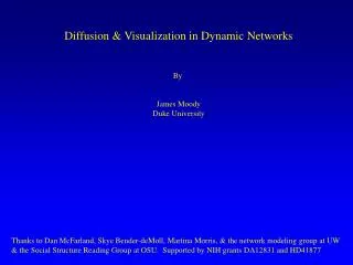
Limits of Diffusion in Dynamic Networks By James Moody Duke University Work reported in this presentation has been supported by NIH grants DA12831, HD41877, and AG024050. Thanks to the Center for Advanced Study in the Behavioral Sciences (CASBS) for support of this work.
The Cocktail Party Problem • Imagine a typical ‘mixer’ party, where one of the guests knows a bit of gossip that everyone would like to know. • Assuming that people tell this gossip to the people they meet at the party: • How many people would eventually hear the gossip? • How long would it take to spread through the group?
The Cocktail Party Problem • Some specifics to narrow down the problem. • 30 people invited, party lasts an hour. • At any given moment in time, you can only carry on a conversation with 3 other people • Guests mingle well – they spend a short time talking to most people, but a long time to a small number (such as their date). • Mingling is somewhat space-based – you talk to the people you bump into, then move on to someone else after a short time. • The bit of gossip moves instantaneously across connected sets (so time-to-diffuse=0).
The Cocktail Party Problem • Some specifics to narrow down the problem. • A (seemingly) simple network problem: record who talks to who, and map the network. Mean distance: 1.99 Diameter: 4 steps
The Cocktail Party Problem • But such an image conflates many temporally distinct events. A more accurate image is something like this: • In general, the graphs over which diffusion happens often: • Have timed edges • Nodes enter and leave • Edges can re-occur multiple times • Edges can be concurrent • These features break transmission paths, generally lowering diffusion potential – and opening a host of interesting questions about the intersection of structure and time in networks.
Outline • Edge timing constraints on diffusion • Returning to the party • Comparing dynamic and static reach profiles • Small-world mechanisms on dynamic graphs • Conditional effectiveness of rewiring • Temporal structure and reachability • Reachability on real structures • Interaction of contact pattern & edge timing • Fundamental (?) unpredictability • A “Mingle Mixing” space of network problems
Edge timing constraints on diffusion “Bits” can only flow forward in time: the finish time of the next step in a path must be > the start time of the last step. 8 - 9 E C 3 - 7 2 - 5 A B 0 - 1 3 - 5 D F A hypothetical Sexual Contact Network
Edge timing constraints on diffusion “Bits” can only flow forward in time: the finish time of the next step in a path must be > the start time of the last step. E C A B D F The path graph for a hypothetical contact network
Edge timing constraints on diffusion Edge time structures are characterized by sequence, duration and overlap. Paths between i and j, have length and duration, but these need not be symmetric even if the constituent edges are symmetric.
Edge timing constraints on diffusion Reachability = 1.0 Implied Contact Network of 8 people in a ring All relations Concurrent
Edge timing constraints on diffusion 1 8 2 7 3 6 5 4 Reachability = 0.71 Implied Contact Network of 8 people in a ring Serial Monogamy (1)
Edge timing constraints on diffusion 2 3 2 1 1 2 2 3 Reachability = 0.57 Implied Contact Network of 8 people in a ring Mixed Concurrent
Edge timing constraints on diffusion 1 2 2 1 1 2 1 2 Reachability = 0.43 Implied Contact Network of 8 people in a ring Serial Monogamy (3)
1 2 2 1 1 2 1 2 Edge timing constraints on diffusion Timing alone can change mean reachability from 1.0 when all ties are concurrent to 0.42. In general, ignoring time order is equivalent to assuming all relations occur simultaneously – assumes perfect concurrency across all relations.
4 2 1 A B C D E F A 0 1 2 2 4 1 B 1 0 1 2 3 2 C 0 1 0 1 2 2 D 0 0 1 0 1 1 E 0 0 0 1 0 2 F 1 0 0 1 0 0 Edge timing constraints on diffusion Path distances need not progress in steps. While (a) is 4 steps from e, and d is 1 step from e, a and e are only two steps apart. This is because a shorter path from a to e emerges after the path from d to e ended.
Edge timing constraints on diffusion The distribution of paths is important for many of the measures we typically construct on networks, and these will be change if timing is taken into consideration: Centrality: Closeness centrality Path Centrality Information Centrality Betweenness centrality Network Topography Clustering Path Distance Groups & Roles: Correspondence between degree-based position and reach-based position Structural Cohesion & Embeddedness Opportunities for Time-based block-models (similar reachability profiles) In general, any measures that take the systems nature of the graph into account will differ.
Edge timing constraints on diffusion • New versions of classic reachability measures: • Temporal reach: The ij cell = 1 if i can reach jthrough time. • Temporal geodesic: The ij cell equals the number of steps in the shortest path linking i to j over time. • Temporal paths: The ij cell equals the number of time-ordered paths linking i to j. • These will only equal the standard versions when all ties are concurrent. • Duration explicit measures • 4) Quickest path: The ij cell equals the shortest time within which i could reach j. • 5) Earliest path: The ij cell equals the real-clock time when i could first reach j. • 6) Latest path: The ij cell equals the real-clock time when i could last reach j. • 7) Exposure duration: The ij cell equals the longest (shortest) interval of time over which i could transfer a good to j. • Each of these also imply different types of “betweenness” roles for nodes or edges, such as a “limiting time” edge, which would be the edge whose comparatively short duration places the greatest limits on other paths.
The Party Revisited Question 1: How does the edge timing affect the overall likelihood that everyone in the party would ultimately hear the gossip? Simulate a cocktail party, manipulate the “mingling” rate and range and compare diffusion over both networks.
The Party Revisited Mingle Range: Mingle Rate: Resulting Density Distributions
The Party Revisited Measuring Diffusion Potential with Network Traces: Cumulative Number of people each node reaches at each step. Dynamic Graph Static Graph Nodes that reach everyone in 4 steps Nodes that never reach everyone Node reaches 9 people in 2 steps Sample “traces” from one run
The Party Revisited Static Density: 0.21 Static Density: 0.24 Static Density: 0.26 Static Density: 0.28 Static Density: 0.23 Static Density: 0.27 Static Density: 0.31 Static Density: 0.36 Static Density: 0.27 Static Density: 0.32 Static Density: 0.35 Static Density: 0.40 Static Density: 0.30 Static Density: 0.34 Static Density: 0.41 Static Density: 0.42 Average (mean of means) reachability & Distance, all runs
The Party Revisited • Timing always lowers the proportion who could be reached in the network and lengthens the distances between connected nodes. • This suggests that diffusion over dynamic networks will tend to be slower than over similar volume static nets. • Note that here we: • a) assumed that diffusion was instant across connected sets • b) assumed complete cliques among conversation groups • c) everyone started at the same time • d) a small group (30 nodes). • If the group is larger, the proportional effects are more dramatic. • If diffusion takes time, edges expire before traversed. • Question 2: Since old paths can’t be joined when actors make new contacts, will the “small world” rewiring effect work?
Small World Mechanisms on Dynamic Graphs • Simulation setup: • Generate a 200 node ring lattice, where every node has 6 ties. • Assign starting times to edges as a random draw from a uniform distribution. Mean concurrency levels are set by compressing or stretching the starting-time distribution. • Each edge is given a duration drawn from a skewed distribution. • Once edge-times are set, randomly rewire the graph by reassigning one end of the edge to a node chosen at random. • Calculate the reachability and mean distance scores for each rewiring. • Repeat 4-5 many times, increasing the number of edges rewired. • Simulation varies the proportion of edges rewired and the level of graph concurrency in the network.
Small World Mechanisms on Dynamic Graphs • The rapid shortening of distance we typically see in small-world simulations does not occur in dynamic networks. • The initial distances are much higher, since many nodes are not reachable. • The rapid decreasing marginal returns to rewiring are much slower • When concurrency is relatively low, the effects of rewiring are nearly linear • When concurrency is relatively high, the characteristic curve starts to emerge, but is much less steep. • Note all of these concurrency levels are non-trivial. Even when only 4% of two-paths in the graph are concurrent, nearly 50% of nodes have at least 1 concurrent edge. • Why?
Small World Mechanisms on Dynamic Graphs • Why do we see this pattern? • Long distant out-reach is rare: • Consider a set of typical reach-paths in a dynamic network with time- disjoint edges: Time e1 e1 p12 = p(e2 > e1) e2 e2 e3 p23 = p(e3 > e2) e4 e3 p34 = p(e4 > e3) P34 < p23 < p12 < 1.0
Small World Mechanisms on Dynamic Graphs • Why do we see this pattern? • Long distant out-reach is rare: • If we allow concurrency & lengthen the duration of edges (proportionate to the observation window): Time e1 e1 p12 = p(e2 > e1) e2 e2 e3 p23 = p(e3 > e2) e4 e3 p34 = p(e4 > e3) Pij is still decreasing, but not as rapidly.
Small World Mechanisms on Dynamic Graphs • Why do we see this pattern? • Long distant out-reach is rare: • If we allow concurrency & lengthen the duration of edges (proportionate to the observation window): Time e1 e1 p12 = p(e2 > e1) e2 e2 e3 p23 = p(e3 > e2) e4 e3 p34 = p(e4 > e3) Pij is constant
Small World Mechanisms on Dynamic Graphs • Why do we see this pattern? • Overlapping paths does not imply joint reach Two starting nodes Medium-concurrency graph
Small World Mechanisms on Dynamic Graphs Two starting nodes Low-concurrency graph
Temporal structure and reachability Structure and Variability Examples thus far lack meaningful network structure. - The party simulation is a (space-constrained) random network - Lattices make all nodes structurally equivalent in the contact pattern Question 3: How does time shape diffusion potential in realistic graphs? a) How much does the contact structure matter? - Minimum possible time-risk - Variance in the variability of time-risk - Individual position vs. network totals b) How much of the diffusion potential can be explained with local rules?
Temporal structure and reachability Structure and Variability Time ordering for the minimum path-density, 2-regular graph. t2 t2 t2 t1 t1 t1 t1 t2 t2 Minimize by weaving early – late – early in paths.
t2 t2 t2 t2 t2 t2 t2 t2 t2 t1 t1 t1 t1 t1 t1 t1 t1 t1 t1 t2 t2 t1 t2 t2 t2 t2 t1 t1 t1 t1 t1 t2 t2 t1 t2 t1 Temporal structure and reachability Structure and Variability Time ordering for the minimum path-density, 2-regular graph. t3 t3 t3 t3 t3 t3 t3 t3 t3 t3 t3 t3 t3 t3 t3 t3 t3 t3 t3 t3 t3 t3 t3 t3 Minimize by weaving early – late – early in paths.
Temporal structure and reachability Structure and Variability Time ordering for the minimum path-density, 2-regular graph. 2 6 10 t2 t1 t2 t1 t2 t1 t3 t3 t3 t3 t3 t3 1 4 5 8 9 12 t3 t2 t1 t2 t1 t2 t1 3 7 11 For a regular graph with constant degree T, you need T times Minimize by weaving early – late – early in paths.
Temporal structure and reachability Structure and Variability • Simulate time structure on a small sample of real graphs. • - These graphs are small walks (~100 nodes) from the soc coauthor network. • - Construct times and durations just as in the SW study • - Record the overall reachability and correlation between node-level centrality • - Examine the reachability pattern relative to minimum possible • - See if we can use some systematic features of the resulting time order to predict reachability
Temporal structure and reachability Structure and Variability 5 example coauthor graphs. (Some of you are in this figure).
Temporal structure and reachability Structure and Variability Distribution of observed concurrency for each network x sim setting … just showing that the structure hasn’t radically affected the overall amount of concurrency
Temporal structure and reachability Structure and Variability Min reachability Proportion of pairs reachable through times
Temporal structure and reachability Structure and Variability Relative Reach – Reachability over minimum possible
Temporal structure and reachability Structure and Variability Relative Reach – Reachability over minimum possible
Temporal structure and reachability Structure and Variability Volume Connectivity Distance Nodes: 83 Mean Deg: 3.04 Density: 0.037 Centralization: 0.237 Mean: 0.398 Diameter: 6 Centralization: 0.321 Largest BC:0.16 Pairwise K: 1.07 Nodes: 148 Mean Deg: 6.16 Density: 0.042 Centralization: 0.187 Mean: 3.59 Diameter: 5 Centralization: 0.312 Largest BC: 0.51 Pairwise K: 1.57 Nodes: 80 Mean Deg: 5.27 Density: 0.067 Centralization: 0.373 Mean: 3.02 Diameter: 5 Centralization: 0.413 Largest BC: 0.33 Pairwise K: 1.34 Nodes: 154 Mean Deg: 3.71 Density: 0.025 Centralization: 0.147 Mean: 4.99 Diameter: 8 Centralization: 0.259 Largest BC: 0.08 Pairwise K: 1.07 Nodes: 128 Mean Deg: 3.39 Density: 0.027 Centralization: 0.205 Mean: 4.55 Diameter: 6 Centralization: 0.301 Largest BC: Pairwise K: 1.06
Temporal structure and reachability Structure and Variability • Networks are structurally cohesive if they remain connected even when nodes are removed 2 3 0 1 Node Connectivity
Temporal structure and reachability Structure and Variability K=1 N=10 1 2 3 4 5 6 7 8 9 0 1 . 3 3 3 2 2 2 2 2 1 2 3 . 3 3 2 2 2 2 2 1 3 3 3 . 3 2 2 2 2 2 1 4 3 3 3 . 2 2 2 2 2 1 5 2 2 2 2 . 4 4 4 4 1 6 2 2 2 2 4 . 4 4 4 1 7 2 2 2 2 4 4 . 4 4 1 8 2 2 2 2 4 4 4 . 4 1 9 2 2 2 2 4 4 4 4 . 1 10 1 1 1 1 1 1 1 1 1 . K=2 N=9 K=3 K=3 N=4 K=4 N=5 K=4 K=2 K=1 Average K = 2.38
Temporal structure and reachability Structure and Variability Net1 Kcon: 1.55 Net3 Kcon: 2.95 Net2 Kcon: 2.43 Kcon: 1.36 Net4 4 clustered networks w. different global connectivity
Temporal structure and reachability Structure and Variability Relative (to min) Reachability
Temporal structure and reachability Structure and Variability Interaction of Structure and Time 7 6 5 4 Mean Relative Reach 3 2 1 1 1.5 2 2.5 3 Pairwise k Connectivity
Temporal structure and reachability Structure and Variability Given the global network effects, does timing interact w. structure at the node level? Define time-dependent closeness as the inverse of the sum of the distances needed for an actor to reach others in the network.* Actors with high time-dependent closeness centrality are those that can reach others in few steps. Note this is directed. Since Dij =/= Dji (in most cases) once you take time into account. *If i cannot reach j, I set the distance to n+1
Temporal structure and reachability Structure and Variability Node-level correlation between closeness centrality & timed closeness (out)