Download
1 / 36
370 likes | 593 Vues
On the Linear Theory of the Land and Sea Breeze. MPO 663 project, Falko Judt based on Rotunno, 1983 Sun and Orlanski, 1981. The Land Sea Breeze…. …. is much more than just and has been studied for quite some time (first quantitative study 1889). Motivation.

E N D
On the Linear Theory of the Land and Sea Breeze MPO 663 project, Falko Judt based on Rotunno, 1983 Sun and Orlanski, 1981
The Land Sea Breeze…. …. is much more than just and has been studied for quite some time (first quantitative study 1889)
Motivation • Derive analytical, linear model for land-sea breeze (okay, it’ll get quite mathy) • Incorporate rotational effects which are important and fundamentally determine behavior of flow • Horizontal scale (How far does it push inland?)
Driving force is diurnal cycle of heating and cooling of land relative to sea • Frequency ω ( 2π/day) • 2 fundamental regimes • f > ω: “classic” flow pattern • f < ω: wave solutions, somewhat strange • f = ω (30˚ latitude) ?? → Singularity!! resonance problem
Atmosphere idealized as rotating, stratified fluid • Characterized by parameters f (Coriolis parameter) and N (Brunt-Väisälä frequency) • N,f = const. • Cartesian 2-D model z x sea land
Equations of motion: shallow, anelastic approx., no friction • BC: w(x,0,t) = 0 b = g
First it had been hypothesized that extent of sea breeze solely based on temp. difference • But: there is a definite internal radius of deformation that determines horizontal scale
Let’s assume heating function Q(x,z,t) known. • Eqs. (1) – (5) can be collapsed into single equation featuring a stream function
gives us solutions of the form Forcing with period ω = 2π/day = 7.292 x 10⁻⁵ s-1 plugging these wave solutions into stream function equation yields
Now simplify N ≈ 10-2 s-1, so N >> ω: We get: Forcing is gradient of heating!
Case 1: f > ω • To get an easier handle on the problem, non-dimensionalize it. • New coordinates: • We get: Height (z) Distance (x) Time (t)
Equation with point source heating can be solved, solution in physical space is: • Ψ is constant on ellipses with the ratio of major to minor axis given by • For increasing static stability N → flatter ellipse of this equation for ellipse diurnal cycle Horizontal scale Vertical scale
It can be shown that the intensity of the flow is inversely proportional to N → Explanation for weaker land breeze at night due to increased stability also shows the dilemma for f → ω
Now let’s make use of some more realistic heating Heating now H, not Q horizontal shape vertical decay
leads to the internal scale of motion. • x0 (scale of land-sea contrast) and z0 (vertical extent) are specified externally • take f = 10-4 s-1, x0 = 1000 m, z0 = 500 m and λH = 73 km just dependent on f, assuming N const.
How does the flow look like? at τ = π/2 (~noon) v (along coast) ψ b u w p http://www.atmos.ucla.edu/~fovell/H98/animations/seabreeze_rotunno_nlin.MOV/
Through Bjerknes’ Circulation theorem following results can be obtained: • Circulation independent of x0 (scale of land-sea contrast) • C independent of N (v ~ N-1, λH ~ N) • C ~ (f2 – ω2)-1 -- Problematic for f → ω
Case 2: f < ω • Redifine xi and beta as follows: • Equation to solve becomes
sunrise Flow concentrated along “rays” of internal-inertial waves noon “Perverse” result: Land breeze during daytime, almost 180˚ out of phase w/ heating sunset
Example Yucatan Peninsula (22˚N): ω = 7.292 x 10⁻⁵ s-1 f = 2 ω sin(22˚) = 5.463 s-1 N = 10-2 s-1 h = 500 m 104 km
Role of friction • According to Circulation Theorem, circulation wave leads temperature wave by 90˚ (max of circulation for max heating, not at sunset (max temperature)) • Observations: Max circulation around mid-afternoon • Friction leads to more realistic phase lags (for both Case 1 and Case 2); • also takes care of singularity (f = ω)
phase lags circulation - heating phase lag for f = 0 • Enhanced friction (α) bring phase lags at different latitudes into line • phase lag ~ 40˚ → observations phase lag heating - temp phase lag for f = ω phase lag for f = 10-4 s-1
Summary • Two fundamentally different solutions for f > ω and f < ω: Elliptic flow pattern vs. internal-inertia waves • Internal radius of deformation which determines inland penetration (dependent on N and f) • Friction necessary to explain “natural” behavior of flow in terms of phase lag (flow-heating) and singular latitude • Observations seem to verify wave solution (Sun and Orlanski, 1981)
Questions? Comments? Complaints?
Inertial Oscillation at 30 N Wind Coriolis Sundown Midnight Sunrise Noon blue slides: John Nielsen-Gammon, TAMU
Tropical Sea Breeze Forces PGF Wind Coriolis Sundown Midnight Sunrise Noon
Tropical Sea Breeze Interpretation • Inertial oscillation is too slow • PGF and CF must be in phase to reinforce each other • Wind oscillates at diurnal frequency
Midlatitude Sea Breeze Forces PGF Wind Coriolis Sunrise Sundown Midnight Noon
Midlatitude Sea Breeze Interpretation • Inertial oscillation is too fast • PGF must be out of phase with CF to slow down inertial oscillation • Wind oscillates at diurnal frequency
Alternative Midlatitude Sea Breeze Interpretation • In midlatitudes, air tries to attain geostrophic balance • Pressure gradient would be associated with alongshore geostrophic flow • Onshore sea breeze is ageostrophic wind trying to produce alongshore geostrophic flow • As if air is entering and exiting an alongshore jet streak
Another Alternative Midlatitude Sea Breeze Interpretation (thanks to Chris Davis) • Sea breeze forcing is diabatic frontogenesis • Frontogenesis produces a direct circulation • Warm air rises, low-level air flows from cold to warm • Intensity of circulation is proportional to the rate of change of the temperature gradient • It really is governed by the Sawyer-Eliassen equation!
Magic Latitudes • At any latitude, L = NH/ (f2 – w2)1/2 • (f2 – w2)1/2 is normally of order 7x10⁻⁵ • For typical H and N, L = 150 km • At 30+/- 1 degrees, (f2 – w2)1/2 is of order 2x10⁻⁵ • For typical H and N, L = 500 km
At 30N or 30S • Diurnal heating cycle resonates with inertial oscillations • Amplitude of response blows up • Horizontal scale blows up • Linear theory blows up