BJT Small-Signal Modeling: Understanding and Application
290 likes | 404 Vues
Explore small-signal modeling of BJT transistors, including diffusion capacitance, transconductance, base currents, and current gain. Learn to analyze circuits and select bias points effectively.

BJT Small-Signal Modeling: Understanding and Application
E N D
Presentation Transcript
Lecture 15:Small Signal Modeling Prof. Niknejad
Lecture Outline • Review: Diffusion Revisited • BJT Small-Signal Model • Circuits!!! • Small Signal Modeling • Example: Simple MOS Amplifier University of California, Berkeley
Large signal Notation Review • Since we’re introducing a new (confusing) subject, let’s adopt some consistent notation • Please point out any mistakes (that I will surely make!) • Once you get a feel for small-signal analysis, we can drop the notation and things will be clear by context (yeah right! … good excuse) small signal Quiescent Point (bias) DC (bias) small signal (less messy!) transconductance Output conductance University of California, Berkeley
Half go left, half go right Wp Diffusion Revisited • Why is minority current profile a linear function? • Recall that the path through the Si crystal is a zig-zag series of acceleration and deceleration (due to collisions) • Note that diffusion current density is controlled by width of region (base width for BJT): • Decreasing width increases current! Density here fixed by potential (injection of carriers) Physical interpretation: How many electrons (holes) have enough energy to cross barrier? Boltzmann distribution give this number. Density fixed by metal contact University of California, Berkeley
Diffusion Capacitance • The total minority carrier charge for a one-sided junction is (area of triangle) • For a one-sided junction, the current is dominated by these minority carriers: Constant! University of California, Berkeley
Diffusion Capacitance (cont) • The proportionality constant has units of time • The physical interpretation is that this is the transit time for the minority carriers to cross the p-type region. Since the capacitance is related to charge: Distance across P-type base Diffusion Coefficient Mobility Temperature University of California, Berkeley
BJT Transconductance gm • The transconductance is analogous to diode conductance University of California, Berkeley
Transconductance (cont) • Forward-active large-signal current: • Differentiating and evaluating at Q = (VBE, VCE ) University of California, Berkeley
BJT Base Currents Unlike MOSFET, there is a DC current into the base terminal of a bipolar transistor: To find the change in base current due to change in base-emitter voltage: University of California, Berkeley
Small Signal Current Gain • Since currents are linearly related, the derivative is a constant (small signal = large signal) University of California, Berkeley
Input Resistance rπ • In practice, the DC current gain F and the small-signal current gain o are both highly variable (+/- 25%) • Typical bias point: DC collector current = 100 A MOSFET University of California, Berkeley
Output Resistance ro Why does current increase slightly with increasing vCE? Collector (n) Base (p) Emitter (n+) Answer: Base width modulation (similar to CLM for MOS) Model: Math is a mess, so introduce the Early voltage University of California, Berkeley
Graphical Interpretation of ro slope~1/ro slope University of California, Berkeley
BJT Small-Signal Model University of California, Berkeley
BJT Capacitors • Emitter-base is a forward biased junction depletion capacitance: • Collector-base is a reverse biased junction depletion capacitance • Due to minority charge injection into base, we have to account for the diffusion capacitance as well University of California, Berkeley
Core Transistor External Parasitic BJT Cross Section • Core transistor is the vertical region under the emitter contact • Everything else is “parasitic” or unwanted • Lateral BJT structure is also possible University of California, Berkeley
Base Collector Emitter Core BJT Model • Given an ideal BJT structure, we can model most of the action with the above circuit • For low frequencies, we can forget the capacitors • Capacitors are non-linear! MOS gate & overlap caps are linear Reverse biased junction Fictional Resistance (no noise) Reverse biased junction & Diffusion Capacitance University of California, Berkeley
Complete Small-Signal Model “core” BJT Reverse biased junctions Real Resistance (has noise) External Parasitics University of California, Berkeley
Circuits! • When the inventors of the bipolar transistor first got a working device, the first thing they did was to build an audio amplifier to prove that the transistor was actually working! University of California, Berkeley
Modern ICs • First IC (TI, Jack Kilby, 1958): A couple of transistors • Modern IC: Intel Pentium 4 (55 million transistors, 3 GHz) Source: Intel Corporation Used without permission Source: Texas Instruments Used without permission University of California, Berkeley
Supply “Rail” A Simple Circuit: An MOS Amplifier Input signal Output signal University of California, Berkeley
Selecting the Output Bias Point • The bias voltage VGS is selected so that the output is mid-rail (between VDD and ground) • For gain, the transistor is biased in saturation • Constraint on the DC drain current: • All the resistor current flows into transistor: • Must ensure that this gives a self-consistent solution (transistor is biased in saturation) University of California, Berkeley
Finding the Input Bias Voltage • Ignoring the output impedance • Typical numbers: W = 40 m, L = 2 m, RD = 25k, nCox = 100 A/V2, VTn = 1 V, VDD = 5 V University of California, Berkeley
Applying the Small-Signal Voltage Approach 1. Just use vGS in the equation for the total drain current iD and find vo Note: Neglecting charge storage effects. Ignoring device output impedance. University of California, Berkeley
Solving for the Output Voltage vO University of California, Berkeley
Small-Signal Case • Linearize the output voltage for the s.s. case • Expand (1 + x)2 = 1 + 2x + x2 … last term can be dropped when x << 1 Neglect University of California, Berkeley
“DC” Small-signal output Linearized Output Voltage For this case, the total output voltage is: The small-signal output voltage: Voltage gain University of California, Berkeley
Plot of Output Waveform (Gain!) Numbers: VDD/ (VGS – VT) = 5/ 0.32 = 16 output input mV University of California, Berkeley
There is a Better Way! • What’s missing: didn’t include device output impedance or charge storage effects (must solve non-linear differential equations…) • Approach 2. Do problem in two steps. • DC voltages and currents (ignore small signals sources): set bias point of the MOSFET ... we had to do this to pick VGS already • Substitute the small-signal model of the MOSFET and the small-signal models of the other circuit elements … • This constitutes small-signal analysis University of California, Berkeley