Download
1 / 76
760 likes | 838 Vues
Explore how the regression equation individualizes predictions beyond estimating population mean. Learn the significance of best fitting lines, slopes, and intercepts in making accurate predictions based on correlation coefficients. Discover the visual representation of relationships and the importance of staying within X score ranges for valid predictions.

E N D
The Regression Equation How we can move beyond predicting that everyone should score right at the mean by using the regression equation to individualize prediction.
Prediction using X scores and r • We are trying to predict, as accurately as possible, the values of Y (or tY) using our knowledge of a person’s X score and of the correlation between X and Y scores. • There are both dangers and advantages to individualizing predictions.
Potential advantages and disadvantages • The potential advantage is the possibility of making more precise, (less wrong) predictions than we would by saying everyone will score right at the estimated population mean, that is, the sample mean. • We are saying, in effect, we know something about this person and this kind of person should score a specific number of points above or below the mean of Y. • The potential danger is that we will make things a good deal worse than they would have been had we stayed with predicting that everyone will score right at the mean.
The definition of the best fitting line plotted on t axes • The best fitting line is a least squares, unbiased estimate of values of Y in the sample. • A “best fitting line” minimizes the average squared vertical distance of Y scores in the sample (expressed as tY scores) from the line. • The generic formula for a line is Y=mx+b where m is the slope and b is the Y intercept. • Thus, any specific line, such as the best fitting line, can be defined by its slope and its intercept.
The intercept of the best fitting line plotted on t axes The origin is the point where both tX and tY=0.000 • So the origin represents the mean of both the X and Y variable • When plotted on t axes all best fitting lines go through the origin. • Thus, the tYintercept of the best fitting line = 0.000.
The slope of and formula for the best fitting line • When plotted on t axes the slope of the best fitting line = r, the estimated correlation coefficient. • To define a line we need its slope and Y intercept • r = the slope and tY intercept=0.00 • The formula for the best fitting line is therefore tY=rtX + 0.00 or tY= rtX
Here’s how a visual representation of the best fitting line (slope = r, tY intercept = 0.000) and the dots representing tX and tY scores might be described. (Whether the correlation is positive of negative doesn’t matter.) • Perfect - scores fall exactly on a straight line. • Strong - most scores fall near the line. • Moderate - some are near the line, some not. • Weak - the scores are only mildly linear. • Independent - the scores are not linear at all.
1.5 Perfect 1.0 0.5 -1.5 -1.0 -0.5 0 0.5 1.0 1.5 0 -0.5 -1.0 -1.5 Strength of a relationship
1.5 1.0 Strong r about .800 0.5 -1.5 -1.0 -0.5 0 0.5 1.0 1.5 0 -0.5 -1.0 -1.5 Strength of a relationship
1.5 1.0 0.5 -1.5 -1.0 -0.5 0 0.5 1.0 1.5 0 -0.5 -1.0 -1.5 Strength of a relationship Moderate r about .500
1.5 1.0 0.5 -1.5 -1.0 -0.5 0 0.5 1.0 1.5 0 -0.5 -1.0 Independent -1.5 Strength of a relationshipr about 0.000
An Important Warning • Notice that each best fitting line starts at the lowest value of X and ends at the highest value of X. • Outside the range of the X scores you saw in your random sample, you can not assume the correlation stays linear. • If it doesn’t, the best fitting line becomes a terrible fit.
1.5 1.0 0.5 -1.5 -1.0 -0.5 0 0.5 1.0 1.5 0 -0.5 -1.0 -1.5 What would happen if you only had pairs with positive tX scores scores when you fit a line here. Outside the range of X scores in your sample, you can’t assume linearity.
Notice what that formula for independent variables says • tY = rtX = 0.000 (tX) = 0.000 • When tY = 0.000, you are at the mean of Y • So, when variables are independent, the best fitting line says that making the best estimate of Y scores in the sample requires you to go back to prediction that everyone will score at the mean of Y (regardless of his or her score on X). • Thus, when variables are independent we go back to saying everyone will score right at the mean. • The visual representation of this is the tY axis, a line in which every score predicts the mean of Y.
Moving from the best fitting line to the regression equation and the regression line.
The best fitting line (tY=rtX) was the line closest to the Y values in the sample. But what should we do if we want to go beyond our sample and use a version of our best fitting line to make individualized predictions for the rest of the population?
tY' = rtX Notice this is not quite the same as the formula for the best fitting line. The formula now reads tY' (read t-y-prime). Not tY. • tY' is the predicted score on the Y variable for every X score in the population falling within the range of X scores observed in our random sample. • Until this point, we have been describing the linear relationship of the X and Y variable in our sample. Now we are predicting tY'scores (estimated ZY scores) for everyone in the population whose X score is in the range of X scores in our random sample.
This is one of the key points in the course; a point when things change radically. Up to this point, we have just been describing scores, means and relationships. We have continued to predict that everyone in the population who was not in our sample will score at the mean of Y. But now we want to be able to make individualized predictions for the rest of the population, the people not in our sample and for whom we can obtain X scores but who don’t have Y scores
In the context of correlation and regression (Ch. 7 & 8), this means making using the correlation between X and Y and someone’s score on the X variable to make predictions of a Y score, from a pre-existing difference among individuals, In Chapter 9 we will determine whether such predictions can be made from the different ways people are treated in an experiment.
Both are somewhat dangerous. Our first rule as scientists is: “Do not increase error.” Individualizing prediction can easily do that. Let me give you an example.
Assume, you are the personnel officer for a mid size company. • You need to hire a typist. • There are 2 applicants for the job. • You give the applicants a typing test. • Which would you hire: someone who types 6 words a minute with 12 mistakes or someone who types 100 words a minute with 1 mistake.
Whom would you hire? • Of course, you would predict that the second person will be a better typist and hire that person. • Notice that we never gave the person with 6 words/minute a chance to be a typist in our firm. • We prejudged her on the basis of the typing test. • That is probably valid in this case – a typing test probably predicts fairly well how good a typist someone will be.
But say the situation is a little more complicated! • You have several applicants for a leadership position in your firm. • But it is not 2006, it is 1956, when we knew that only white males were capable of leadership in corporate America. • That is, we all “knew” that leadership ability is correlated with both gender and skin color, white and male are associated with high leadership ability and darker skin color and female gender with lower leadership ability.
In 1956, it would have been just as absurd to hire someone of color or a woman for a leadership position as it would be to hire the bad (6-words-a- minute-with-12-mistakes) typist now. Everyone knew that 1) they couldn’t do the job and/or that even if they had some talent 2) no subordinate would be comfortable following him or her. • We now know this is absurd, but lots of people were never given a chance to try their hand at leadership, because of a socially based pre-judgment that you can now see as obvious prejudice.
We would have been much better off saying that everyone is equal, everyone should be predicted to score at the mean. • Pre-judgments on the basis of supposed relationships between variables that have no real scientific support may well be mere prejudice. • In the case we just discussed, they cost potential leaders jobs in which they could have shown their ability. That is unfair.
We would have been much better off saying that everyone is equal, everyone should be predicted to score at the mean. • Moreover, by excluding such individuals, you narrow the talent pool of potential leaders. The more restricted the group of potential leaders, the less talented the average leader will be. • This is why aristocracies don’t work in the long run. The talent pool is too small.
So, to avoid prejudice you must start with the notion that everyone will score at the mean of Y no matter how they scored on the X variable, the predictor variable.In math language you have to predict that ZY'~tY' =0.00 for every value of XHow can you do that?To figure it out, look carefully at the regression equation: tY' = rtX
If tY' = rtX, the only way that tY' will always equal 0.00 is when r = 0.000. (Actually, in this case we are using a theory that X and Y scores can not be used to predict each other. When you are talking theory, the proper form of the regression equation is Artie’s sister, Rosie (ZY' = rhoZX) Thus, to predict that everyone in the population will score at the mean of Y (ZY' = 0.00), you have to hypothesize that rho = 0.000.
So, to avoid the possibility of disastrous mistakes and prejudice,only if you can disprove the notion that rho = 0.000 and no other time,should you make any other prediction than “Everyone is equal, everyone should be predicted to score right at the mean”.
In regression analysis,we call the hypothesis that rho=0.000 the null hypothesis The symbol for the null hypothesis is H0. We will see the null hypothesis many times during the rest of this course. Though it appears in several forms, the null hypothesis is the only hypothesis that you will learn to test statistically in this course.
To use the regression equation to predict Y scores for the part of the population that was not in your random sample, you must falsify and reject the null. • You must start with the assumption that rho=0.000 and that the best prediction is that everyone will score right at the meanunless you can prove otherwise. • Proof does not mean beyond any doubt, it means beyond a reasonable doubt. • There have to be five chances in 100 or less of our sample looking as it does, if the null were to be true, for us to declare the null false and reject it.
Can you say with absolute certainty that the null hypothesis is wrong? • NO! NEVER! However, you can say that there are 5 or fewer chances in 100 that you will get a correlation as strong as the one you found in your random sample, when the null is true (p<.05) • If your results are particularly strong, you may be able to brag by saying that there is one or fewer chances in 100 of finding your data when the null is true (p<.01). • But there is always some chance that you have simply obtained an unusual random sample and that the null really is true.
Statistical Significance • In either event (p<.05 or p<.01) your results are considered statistically significant and you must consider the null so wrong about the data you obtained from your random sample that you must discard it. • You then use the regression equation to make predictions of Y scores using each person’s X score and the correlation of X and Y in your random sample.
Remember when your results are statistically significant, you have falsified and must reject the null hypothesis.
You can’t use the regression equation to predict tY when you have an X score outside the range of scores you observed in your random sample. • The one thing you know about someone with an X score outside the range of scores in your random sample is that YOU KNOW NOTHING ABOUT SUCH PEOPLE. You never saw one before.
The regression line has end points, just like the best fitting line. • Notice that each regression starts at the lowest value of X and ends at the highest value of X. • Outside the range of the X scores you saw in your random sample, you can not assume the correlation stays linear. • If it doesn’t, your predictions of Y can become absurdly wrong.
Like the example in your book: • Imagine you measured the height of girls between 2 and 14, with a mean age of 8.00 and a standard deviation of 3 years. Mean height was 48” with a standard deviation of 8”. • You find a correlation of +0.600 between height and age. Older girls tend to be taller. • So, the regression equation is tY' = 0.600 tX • This allows you to predict that at 5 years the average girl will be 40 inches tall, while at age 14 girls will average 64” tall.
Now you want to predict the height of the average 83 year old. • Let’s say you forget the rule about not predicting outside the range of X scores in your sample. • If we translate 83 to a tX score, you get • tX=(83-8)/3 = 25.00 • Using the regression equation, you would predict that tY' = .6(25.00) =15.00 • Y' = Ybar+ tY‘(sY) = 48” + 15(8”) =168” • You just predicted the average 83 year old will be 14 feet tall.
What went wrong. • You assumed linearity outside the range of scores you had seen on the X variable (age). • You saw kids 2-14. They are growing and within that age group age and height have a positive, linear relationship • But by 14 or 15 growth stops and the curve goes from rising to flat, eventually going down a little. • It doesn’t stay linear. It becomes curvilinear as soon as you include kids 15 and over and adults along with kids.
1.5 1.0 0.5 -1.5 -1.0 -0.5 0 0.5 1.0 1.5 0 -0.5 -1.0 -1.5 So, outside the range of X scores in your sample, you can’t assume linearity. Here mean age = 12 s= 5.00
Predict they will score right at the mean of Y • Remember, the one thing you know about someone with an X score outside the range of scores in your random sample is that YOU KNOW NOTHING ABOUT SUCH PEOPLE. You never saw one before. • So you do what we always do when we don’t know anything about someone: We predict they will be average, that they will score right at the mean of Y.
Confidence intervals around rhoT • In Chapter 6 we learned to create confidence intervals around muT that allowed us to test a theory. • To test our theory about mu we took a random sample, computed the sample mean and standard deviation, and determined whether the sample mean fell into that interval. • If the sample mean fell into the confidence interval, there was some support for our theory, and we held onto it.
Confidence intervals around muT • The interesting case was when muT fell outside the confidence interval. • In that case, the data from our sample falsified our theory, so we had to discard the theory and the estimate of mu specified by the theory
If we discard a theory based prediction, what do we use in its place? • Generally, our best estimate of a population parameter is the sample statistic that estimates it. • Our best estimate of mu has been and is the sample mean, X-bar. • Since X-bar fell outside the confidence interval, we discarded our theory about the value of mu. • If we reject the theory (hypothesis) about mu, we must go back to using X-bar, the sample mean that fell outside the confidence interval and falsified our theory, as our best (least squares, unbiased, consistent estimate) of mu.
To test any theory about any population parameter, we go through similar steps: • We theorize about the value of the population parameter. • We obtain some measure of the variability of sample-based estimates of the population parameter. • We create a test of the theory about the population parameter by creating a confidence interval, almost always a CI.95. • We then obtain and measure the parameter in a random sample.
Which hypothesis about rho (the population correlation coefficient) do we always test in this way. • THE NULL HYPOTHESIS • The null says that there is no relationship between any two variables we chose to study, in the population as a whole. Mathematically, we would say that rho=0.000. A Corollary: If rho = 0.000, any nonzero correlation found in a random sample is simply a poor estimate or rho. Thus, whatever nonzero correlation you found in the sample is illusory. It is simply a mediocre estimate of zero.
Testing the null hypothesis (rho = 0.000) in correlation and regression