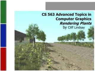
CS 563 Advanced Topics in Computer Graphics Rendering Plants
310 likes | 480 Vues
CS 563 Advanced Topics in Computer Graphics Rendering Plants. by Cliff Lindsay. Overview. Eco Systems – LOD 3 (high level) Plant Structures – LOD 2 (medium level) Plant, Light Interaction – LOD 1 (close up). Prerequisites. L-Systems Terminology: PDF – Probability Density Function

CS 563 Advanced Topics in Computer Graphics Rendering Plants
E N D
Presentation Transcript
CS 563 Advanced Topics in Computer GraphicsRendering Plants by Cliff Lindsay
Overview • Eco Systems – LOD 3 (high level) • Plant Structures – LOD 2 (medium level) • Plant, Light Interaction – LOD 1 (close up)
Prerequisites • L-Systems Terminology: PDF – Probability Density Function Self-thinning – plant mortality due to competition
L-systems • String rewriting mechanism that reflects biological motivation. L-system Components: • Alphabet • Axiom – start string • Productions • Example: • Alphabet: {F, +, -} where “F” = move forward, “+” = turn degree, “-” = turn – degrees • Axiom: F • Production: F F-F++F-F 1st generation S = F-F++F-F 2nd generation S = F-F++F-F-F-F++F-F++F-F-F++F-F Examples from [Przem90]
Plant Distributions in Eco Systems • Positioning • L – systems • Self-thinning Curve • Multi-species Competitive Models
Positioning Initial Task Hierarchy: • Terrain Generation • Initial Random Placement • Plant Ecological Characteristics (growth, reproduction rates, terrain preferences, light tolerances, etc) • Grow Plants Iteratively (life cycle) • Result is a distribution of plants. [Deussen98]
Positioning Positioning Improvements: • Clustering using Hopkins Index • Environmental factors mimicked by Hopkins: • Favorable growth areas • Seed propagation (seeds fall close to parents) • Other mechanisms [Brendan02] [Brendan02]
Scene Modeling Multi-set L-system (L-system extension): • Allows for sets of Axioms • Productions work on Multi-sets of Strings • Allows for Fragmentation of plant Why is the extension necessary?: • Operations for multiple plants at once • Dynamically add or remove plants (birth, death) • Communication Between Plants and Environment Has All The Regular Stuff Too: • Size • Position • Allows for growth
Scene Modeling • Individual Circles Represent ecological of a Plant (previous, and next slide) • Biologically Motivated Rules Govern Outcomes of interaction Between Circles • Self-thinning Curve: [Deussen98]
Self-Thinning • Competition: • Among Plants of Same Age & Species • Limited Resources (water, minerals, light) • Larger plants dominate smaller • We need L-system extension to include self-thinning [Brendan02] [Brendan02]
Multi-species Competitive Models Multi-set L-system: Additional Parameters • Parameter For Species Additional Productions • Plant Domination, and Competition • Shading due to Domination • Reduction of Resources
Multi-Species Result Step 1 Step 2 Step 3 Step 4 [Brendan02]
Plant Structures Components of Plants Models: • Primitives • Parameters • Special Cases • Ideas Based on [WEBER95]
Plant Primitives Primitives: • Stems • Curves • Length • Splits • Leaves • Orientation • Color • Shape • Each Stem has a unique coordinate system [weber02]
Plant Parameters Additional Parameters: • Taper • Split Angle • Radius [weber02]
Special Parameters Special Tree Parameters: • Pruning • Wind Sway • Vertical Attraction • Leaf Orientation [weber02]
Tree Structure Results [Weber95]
Tree Structure Results [Weber95]
Treal Tree Render Demo • Go To Treal Demo (2-3 minutes)
Light Interaction with Plant Tissue Models • ABM – Our Focus • Plate models • N-Flux Models Terminology: SPF – Scattering Probability Function ABM – Algorithmic BDF Model BDF – AKA: BSSDF, Bidirectional Surface-scatering Distribution Function Oblate – round or elliptical geometry that is flat at poles
What Does ABM Do? • Computes Light interaction: • Surface Reflectance • Subsurface Reflectance • Transmittance • Absorption • Incorporates Biological Factors into theses computations
Scattering Probability Functions Leaf Model rays in up direction rays in down direction Interface: 1 epidermis mesophyll 2 air 3 epidermis 4 Picture Recreated from [Bara97]
Where 1, 2 = uniform random numbers [0, 1] Determine Surface Reflectance • e– corresponds to polar angle displacement • e– corresponds to the Azimutal angle displacement • Epidermal Cells With Large oblateness make for a reflection closer to specular distribution. [Bara97,Bara98]
Where 1, 2 = uniform random numbers [0, 1] Subsurface Reflectance and Transmittance • m– corresponds to polar angle displacement • m– corresponds to the Azimutal angle displacement • Light passing to the Mesophyll Layer becomes randomized, thus diffuse [Bara97,Bara98]
Absorption • Beer’s Law of absorption • P = path length of ray through cell medium (collision w/ cell) • P tm where tm = thickness of the Mesophyll cells, ray is absorbed Where: = uniform random number [0,1] Ag = global absorption coefficient = angle between ray direction & normal [Bara97]
Conclusion of Simplified ABM • Color mapping of CIE XYZ -> SMPTE • Comparison from Measured Sample and ABM model spectra [Bara97]
Resultant ABM Images [Glad98]
Plate Models • Simple Slab(s) of Diffusing and Absorbing Material • N – plates separated by N-1 air spaces • Parameters: • Amount of water and chlorophyll • # of plates [Jacq01]
N-Flux Models • Based on Kubelka-Munk theory of reflectance • Io = incident light intensity • Applied to a Single slab of diffuse and absorbing material [Jacq01]
Insights, Future, and Cool Stuff • Virtual Terrain Project http://www.vterrain.org/Plants/index.html • More Research Needed for specific BRDFs of plants • Treal Tree Render using Jason Weber and Joseph Penn’s tree models[weber95] and Povray (Demo Software) http://members.chello.nl/~l.vandenheuvel2/Treal/
References • Brendan Lane, Przemyslaw PrusinkiewiczGenerating spatial distributions for multilevel models of plant communities. Proceedings of Graphics Interface 2002. • Oliver Deussen, Pat Hanrahan, Bernd Lintermann, Radomir Mech, Matt Pharr, and Przemyslaw Prusinkiewicz. Realistic modeling and rendering of plant ecosystems. Proceedings of SIGGRAPH 98. • Jason Weber, joeseph Penn, Creation and Rendering of Realstic Trees,Proceedings of the 22nd annual conference on Computer graphics and interactive techniques September 1995. • G. V.G. Baranoski, J. G. Rokne, Simplified model For Light Interaction with Plant Tissue, Proceedings of the Eighth International Conference on Computer Graphics and Visualization - GraphiCon'98, Moscow, Russia, September, 1998 • G. V. G. Baranoski, J. G. Rokne. An algorithmic reflectance and transmittance model for plant tissue. Computer Graphics Forum (EUROGRAPHICS Proceedings), 16(3):141–150, September 1997. • S. Jacquemoud,S.L.Ustin (2001),Leaf optical properties: A state of the art, in Proc. 8th Int. Symp. Physical Measurements & Signatures in Remote Sensing, Aussois (France), 8-12 January 2001 • Przemyslaw Prusinkiewicz, Aristad Lindenmayer, “The Algorithmic Beauty of Plants”, Springer Verlag, 1990