PID Controller
PID Controller. Different Types of Feedback Control On-Off Control This is the simplest form of control. Proportional Control

PID Controller
E N D
Presentation Transcript
Different Types of Feedback Control On-Off Control This is the simplest form of control.
Proportional Control A proportional controller attempts to perform better than the On-off type by applying power in proportion to the difference in temperature between the measured and the set-point. As the gain is increased the system responds faster to changes in set-point but becomes progressively underdamped and eventually unstable. The final temperature lies below the set-point for this system because some difference is required to keep the heater supplying power.
Proportional, Derivative Control The stability and overshoot problems that arise when a proportional controller is used at high gain can be mitigated by adding a term proportional to the time-derivative of the error signal. The value of the damping can be adjusted to achieve a critically damped response.
Proportional+Integral+Derivative Control Although PD control deals neatly with the overshoot and problems associated with proportional control it does not cure the problem with the steady-state error. Fortunately it is possible to eliminate this while using relatively low gain by adding an integral term to the control function which becomes
The Characteristics of P, I, and D controllers A proportional controller (Kp) will have the effect of reducing the rise time and will reduce, but never eliminate, the steady-state error. An integral control (Ki) will have the effect of eliminating the steady-state error, but it may make the transient response worse. A derivative control (Kd) will have the effect of increasing the stability of the system, reducing the overshoot, and improving the transient response.
Proportional Control By only employing proportional control, a steady state error occurs. Proportional and Integral Control The response becomes more oscillatory and needs longer to settle, the error disappears. Proportional, Integral and Derivative Control All design specifications can be reached.
CL RESPONSE RISE TIME OVERSHOOT SETTLING TIME S-S ERROR Kp Decrease Increase Small Change Decrease Ki Decrease Increase Increase Eliminate Kd Small Change Decrease Decrease Small Change The Characteristics of P, I, and D controllers
Tips for Designing a PID Controller 1. Obtain an open-loop response and determine what needs to be improved 2. Add a proportional control to improve the rise time 3. Add a derivative control to improve the overshoot 4. Add an integral control to eliminate the steady-state error • Adjust each of Kp, Ki, and Kd until you obtain a desired overall response. Lastly, please keep in mind that you do not need to implement all three controllers (proportional, derivative, and integral) into a single system, if not necessary. For example, if a PI controller gives a good enough response (like the above example), then you don't need to implement derivative controller to the system. Keep the controller as simple as possible.
Open-Loop Control - Example num=1; den=[1 10 20]; step(num,den)
Proportional Control - Example The proportional controller (Kp) reduces the rise time, increases the overshoot, and reduces the steady-state error. MATLAB Example Kp=300; num=[Kp]; den=[1 10 20+Kp]; t=0:0.01:2; step(num,den,t) K=100 K=300
Proportional - Derivative - Example The derivative controller (Kd) reduces both the overshoot and the settling time. MATLAB Example Kp=300; Kd=10; num=[Kd Kp]; den=[1 10+Kd 20+Kp]; t=0:0.01:2; step(num,den,t) Kd=10 Kd=20
Proportional - Integral - Example The integral controller (Ki) decreases the rise time, increases both the overshoot and the settling time, and eliminates the steady-state error MATLAB Example Kp=30; Ki=70; num=[Kp Ki]; den=[1 10 20+Kp Ki]; t=0:0.01:2; step(num,den,t) Ki=70 Ki=100
Example - Practice Consider the following configuration:
Lead or Phase-Lead Compensator Using Root Locus A first-order lead compensator can be designed using the root locus. A lead compensator in root locus form is given by where the magnitude of z is less than the magnitude of p. A phase-lead compensator tends to shift the root locus toward the left half plane. This results in an improvement in the system's stability and an increase in the response speed. When a lead compensator is added to a system, the value of this intersection will be a larger negative number than it was before. The net number of zeros and poles will be the same (one zero and one pole are added), but the added pole is a larger negative number than the added zero. Thus, the result of a lead compensator is that the asymptotes' intersection is moved further into the left half plane, and the entire root locus will be shifted to the left. This can increase the region of stability as well as the response speed.
Lead or Phase-Lead Compensator Using Root Locus In Matlab a phase lead compensator in root locus form is implemented by using the transfer function in the form numlead=kc*[1 z]; denlead=[1 p]; and using the conv() function to implement it with the numerator and denominator of the plant newnum=conv(num,numlead); newden=conv(den,denlead);
Lag or Phase-Lag Compensator Using Root Locus A first-order lag compensator can be designed using the root locus. A lag compensator in root locus form is given by where the magnitude of z is greater than the magnitude of p. A phase-lag compensator tends to shift the root locus to the right, which is undesirable. For this reason, the pole and zero of a lag compensator must be placed close together (usually near the origin) so they do not appreciably change the transient response or stability characteristics of the system. When a lag compensator is added to a system, the value of this intersection will be a smaller negative number than it was before. The net number of zeros and poles will be the same (one zero and one pole are added), but the added pole is a smaller negative number than the added zero. Thus, the result of a lag compensator is that the asymptotes' intersection is moved closer to the right half plane, and the entire root locus will be shifted to the right.