Quantify prediction uncertainty (Book, p. 174-189)
170 likes | 315 Vues
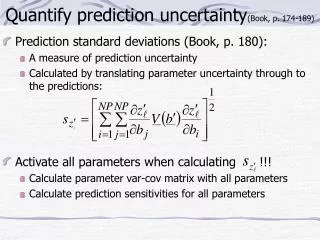
Quantify prediction uncertainty (Book, p. 174-189). Prediction standard deviations (Book, p. 180): A measure of prediction uncertainty Calculated by translating parameter uncertainty through to the predictions: Activate all parameters when calculating !!!

Quantify prediction uncertainty (Book, p. 174-189)
E N D
Presentation Transcript
Quantify prediction uncertainty(Book, p. 174-189) • Prediction standard deviations (Book, p. 180): • A measure of prediction uncertainty • Calculated by translating parameter uncertainty through to the predictions: • Activate all parameters when calculating !!! • Calculate parameter var-cov matrix with all parameters • Calculate prediction sensitivities for all parameters
Quantify prediction uncertainty • Linear confidence and prediction intervals (p. 176-177) • Intervals can be individual or simultaneous • Form: confidence interval prediction interval Prediction intervals account for ‘measurement’ error. Use to compare simulated results to field measurements. a is the significance level, c(a) is the critical value and is different for different types of intervals (Table 8.1, p. 176).
Individual vs. Simultaneous Intervals • Individual linear intervals • Defined as an interval that has a specified probability of containing the true predicted value. • Exact for correct, linear models with normally distributed residuals. • The more these requirements are violated, the less accurate the intervals become. • Simultaneous linear intervals • On two or more predictions, each has a specified probability of containing the true value. • Always ≥ linear intervals, because of greater difficulty in defining intervals that simultaneously include true values of two or more predictions. Largest intervals are for case where # of predictions= # of parameters • Common types: Bonferoni & Sheffé
Exercise 8.2a: Calculate linear confidence intervals on predicted advective transport • Linear confidence intervals can be computed in UCODE_2005 using program Linear_Uncertainty.exe. • Linear_Uncertainty uses V(b) from the regression run output, along with information from an extra ucode run with the prediction conditions (for computing prediction sensitivities) to calculate prediction standard deviations. • Then it calculates the different types of individual and simultaneous intervals using the appropriate statistics.
Calculating linear intervals with UCODE_2005. From Poeter +, 2005, p. 158)
Linear Intervals Do Exercise 8.2a (p. 208-209) and the Problem, including answering Question 5: What is the uncertainty in the predictions? • Correction to book: p. 208, second line from the bottom, should read “Answer Question 5…”
Figure 8.15a, p. 210 Linear Individual Results of Exercise 8.2aLinear Confidence Intervals for Question 5: What is the prediction uncertainty? Linear Simultaneous (Scheffe d=NP) Figure 8.15b, p. 210
Results of Exercise 8.2a(continued)Linear Confidence Intervals for Question 5: What is the prediction uncertainty? Figure 8.16, p. 211
Method involves finding the minimum and maximum predicted value on a confidence region for the parameters, which is defined as (book, p. 178) S(b) S(b’) + (s2 x crit) + a crit=critical value Nonlinear Intervals Maximum prediction Minimum prediction Developed by Vecchia and Cooley (1987, WRR) Each limit of each interval requires a regression run that is often more difficult than the regression runs used for calibration.
Calculating nonlinear intervals with UCODE_2005. Modified from Poeter +, 2005, p. 193)
Nonlinear Intervals • Do exercise 8.2b • Computer instructions: the input files are provided for you in initial\ex8\ucode-opr-ppr-runs\ex8.2b directory, as noted in the computer instructions. • The nonlinear intervals are in ex8.2b._intconf
Figure 8.15c, p. 210 Nonlinear Individual Results of Exercise 8.2bNonlinear Confidence Intervals for Question 5: What is the prediction uncertainty?Do the Problem on p. 212 Nonlinear Simultaneous (Scheffe d=NP) Figure 8.15d, p. 210
Linear Simultaneous (Scheffe d=NP) Linear Individual Figure 8.15a, p. 210 Figure 8.15, p. 210 Nonlinear Simultaneous (Scheffe d=NP) Nonlinear Individual
Our Final Analysis and the County Decision • Our Analysis • Though it looks likely that the particle goes to the well, results are not conclusive. • Consider using parameter values for which the particle goes to the river in an advective-dispersive model to analyze concentrations at the well. If concentrations high, results become more conclusive. • County decision • No additional modeling right now • Wait for the new data and use it to recalibrate
Monte Carlo Analysis (Book, p. 185-189) • Change some aspect of model input, run model, evaluate selected changes in model results. • Can change parameter values, definition of hydrogeology, etc. • When changing parameter values, can generate new sets from V(b) if model was calibrated by regression. For changing hydrogeology, a common geostatistical approach is ‘simulation’, which uses kriging as part of the method. • Can just do forward simulations, or can involve inverse modeling as well. • Commonly need to do numerous model runs to obtain enough ‘data’ to make supportable conclusions. This is now often feasible, with the level of computational power in PCs. • Results commonly displayed as histograms showing distribution of model output values; can also calculate statistics from the results, such as means and variances. • Suggestion: only use sets of generated parameter values that produce a reasonable fit to the calibration data (Beven)
Can confidence intervals replace traditional sensitivity analysis? (p. 184-185) • Traditional sensitivity analysis • quantify uncertainty in the calibrated model caused by uncertainty in the estimated parameter values • change hydraulic conductivity, storage, recharge and boundary conditions systematically within previously established plausible range • Weaknesses of traditional method • Plausible range does not reflect significant information provided through model calibration. Results exaggerate uncertainty. • Suggested method to account for parameter correlation exacerbates this exaggeration.
Can confidence intervals replace traditional sensitivity analysis? • Weaknesses of both methods • Only consider uncertainty in the parameter values. • Uncertainty in model construction generally neglected entirely • Advantages of confidence intervals • Account for information provided through the modeling process.