Download
1 / 36
360 likes | 558 Vues
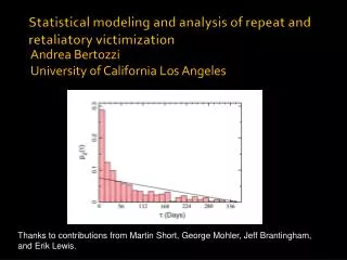
Statistical modeling and analysis of repeat and retaliatory victimization. Andrea Bertozzi University of California Los Angeles. Thanks to contributions from Martin Short, George Mohler, Jeff Brantingham, and Erik Lewis. Short et al J. Quant. Crim. 2009.

E N D
Statistical modeling and analysis of repeat and retaliatory victimization Andrea Bertozzi University of California Los Angeles Thanks to contributions from Martin Short, George Mohler, Jeff Brantingham, and Erik Lewis.
Short et al J. Quant. Crim. 2009 repeat crime is much more likely to happen in a short interval of time after the first event
Event Dependence • burglars return to places to replicate the successes of and/or exploit vulnerabilities identified during previous offenses: “I always go back [to the same places] because, once you been there, you know just about when you been there before and when you can go back. An every time I hit a house, it’s always on the same day [of the week] I done been before cause I know there ain’t nobody there. “ (Subject No. 51) Wright and Decker Burglars on the Job (1996: 69)
Crime Clusters in Space & Time On right, histogram of times between pairs of burglaries separated by 200m or less. On the left, similar histogram for Southern California earthquake (magnitude 3.0 or greater) pairs separated by 220km or less.
Random Event HypothesisM. B. Short et al J. Quant. Crim. 2009. • Events occur entirely at random, defining a stochastic process where each event occurs independently of prior events. • Mathematically, such a phenomenon can be modeled as a Poisson process characterized by a rate parameter l, representing the expected number of events per unit time. • the probability that one burglary occurs within a time interval t to t + dt is given by • The probability that k burglaries occur is given by the general Poisson distribution • The probability that no events occur within a time interval dt, then, is given by
REH and distribution of time intervals between exact repeat events. • The time T1 until the first event occurs • Probability that first event occurs between times t and t+dt • Poisson process probability density function for time interval between events
Probabilities of events with different rate constants • Suppose we have different types of events associated with different locations, e.g. residential burglaries whose rates vary by spatial location. Then the composite probability is • Where wi is the fraction of homes exhibiting rate constant li.
Comparison of repeat probabilities using ``moving window’’ count – Longbeach Burglary Data • Fit to With N = 3
Interpretation of Data • At first glance the good fit with N=3 suggests that the Long Beach data satisfies the REH. • However it turns out that only a fraction of the total number of houses fit into the N=1, N=2, N=3 bins as determined by “house order” the total number of times burgled during the time period of evaluation. • Suggests we need another method for measuring repeat victimization.
Fixed window method • Parameter free method • Pick a fixed window time period D • Probability distribution of time intervals between victimization for order 2 homes (homes that have exactly two events during this window perios, assuming REH):
Example with Long Beach data • Comparison to REH shown as black line. • D=364
Crime Clusters in Space & Time On right, histogram of times between pairs of burglaries separated by 200m or less. On the left, similar histogram for Southern California earthquake (magnitude 3.0 or greater) pairs separated by 220km or less.
Self-exciting point process models in Seismology • A space-time point process is characterized by its conditional intensity given a history Ht • Epidemic Type Aftershock Sequence models (ETAS) divide earthquakes into two categories: background events and aftershock events.
Formula for conditional intensity • Background events occur according to a stationary process m with magnitudes distributed independently of m with probability j(M). • Each of these earthquakes then elevates the risk of aftershocks and the elevated risk spreads in space and time according to the kernel g(t; x; y;M).
Parameter estimation • Parameter selection for ETAS models is most commonly accomplished through maximum likelihood estimation, where the log likelihood function (Daley and Vere-Jones, 2003), is maximized over all parameter sets .
Akaike Information Criterion • Measure of goodness of fit of a statistical model – used for model selection • AIC=2K-2ln(L) where K is the number of parameters in the model and L is the maximized value of the likelihood function of the model. • The AIC methodology attempts to find the model that best explains the data with a minimum of free parameters. • If model errors are normally and independently distributed, then AIC is equivalent to 2K+n[ln(RSS)], RSS is residual sum of squares (difference between data and model prediction) where n is number of observations. • Preferred model has the lowest AIC value.
Gang networks and self-excitation Rivalry network among 29 street gangs in Hollenbeck, Los Angeles Tita et al. (2003)
a general statistical structure • event dependence is a common process driving repeat victimization across all crime types • specific behavioral mechanism—street smarts/street justice—may differ in detail, but outcome is the same • Hawkes Process is a flexible representation of self-excitation
Hawkes Process self-excitation rivalry intensity background rate of violence time since the most recent incident retaliation strength retaliation duration
actual Mike Egesdal, Chris Fathauer, Kym Louie, and Jeremy Neuman, Statistical Modeling of Gang Violence in Los Angeles, submitted to SIURO. simulated
Overview of Hollenbeck Gangs Here k0 is the expected number of retaliations per attack, 1/w is the expected waiting time for retaliation (in days)
Comparison with Crime Hotspot Maps Percentage of crimes predicted vs percentage of cells flagged for 2005 burglary (left) and 2007 robbery (right). Curve for CHM is point wise max over a variety of hotspot map prediction methods discussed in the criminological literature.
Current Research: Insurgencies n events Najaf, Iraq inter-event times Najaf, Iraq Data from Iraq Body Count, analysis by Erik Lewis, UCLA
Models with time dependent background rate • Iraqi data shows a clear temporal dependence on background rate likely linked to troop presence. • We consider several models for change in background rate : • (a) step model, • (b) linear increase, • (c ) variable bandwidth kernel smoothing.
Parameter estimation using maximum likelihood • Example – linear background rate
Data from Iraq Body Count • Time period: March 20, 2003 – Dec. 31, 2007 • 15,977 events • Start date, end date, min and max # deaths, town and/or district. • In the analysis no distinction is made between different # deaths per event. • Do not distinguish between type of event (e.g. IED or gunfire). • Only consider start date. (93% of events have same start/end date)
Najaf data – linear model A histogram of all 149 events in Najaf with 30 bins is plotted on the left. The estimated fit with a linear background rate is plotted on the right (the jagged curve). The linear fit without self excitation is shown as well.
References • M.B. Short, M.R. D'Orsogna, P.J. Brantingham, and G.E. Tita, Measuring and modeling repeat and near-repeat burglary effects, J. Quant. Criminol.25 (2009). • G.O. Mohler, M.B. Short, P.J. Brantingham, F.P. Schoenberg, and G.E. Tita, Self-exciting point process modeling of crime, preprint (2010). • Feller W (1968) An introduction to probability theory and its applications, 3rd edn., vol 1. Wiley, New York. • Daley, D. and Vere-Jones, D. (2003). An Introduction to the Theory of Point Processes, 2nd edition. New York: Springer. • Statistical Modeling of Gang Violence in Los Angeles Mike Egesdal, Chris Fathauer, Kym Louie, Jeremy Neuman, SIAM J. Undergraduate Research Online, 2010. • Mark Allenby, Kym Louie, and Marina Masaki, project report, Tim Lucas mentor, A Point Process Model for Simulating Gang-on-Gang Violence , 2010 REU program at UCLA. • E. Lewis, G. Mohler, P. J. Brantingham, and A. L. Bertozzi, Self-Exciting Point Process Models of Civilian Deaths in Iraq, preprint 2010.
More references • Johnson, S. (2008). Repeat burglary victimisation: a tale of two theories. IEEE Trans. Automatic Control , 4 , 215-240. • Townsley, M., Johnson, S. D., & Ratclie, J. H. (2008). Space time dynamics of insurgent activity in Iraq. Security Journal , 21 , 139-146. • Iraq Body Count. (2008). Iraq body count. http://www.iraqbodycount.net. • Akaike, H. (1974). A new look at the statistical model identication. IEEE Trans. Automatic Control , AC-19 , 716-723. • Akaike, H. (1973). Information theory and an extension of the maximum likelihood principle. Budapest: Akademiai Kiado.