Download
1 / 11
110 likes | 205 Vues
Explore how fiscal and monetary policies affect interest rates and national income in the short run using the IS-LM model. Learn about government purchases, taxes, money supply, and aggregate demand.

E N D
Aggregate Demand II The Economy in the Short-Run Source: "Macroeconomics", Mankiw, 4th Edition: Chapter 11, Fifth Edition: Chapter 11
Introduction • In the last chapter we derived the IS and LM curves • IS curve: represents the equilibrium in the market for goods and services • LM Curve: represents the equilibrium in the market for real money balances • IS and LM curves together determine the interest rate and the national income in the short run, when the price level is fixed Source: "Macroeconomics", Mankiw, 4th Edition: Chapter 11, Fifth Edition: Chapter 11
Introduction • Here, we examine potential causes of fluctuations in national income • Use IS-LM model to see: • How changes in government purchase and taxes (i.e. fiscal policy) influence the interest rate and national income. Note: Government purchases and taxes are the exogenous variables and interest rate and national income are the endogenous variables Source: "Macroeconomics", Mankiw, 4th Edition: Chapter 11, Fifth Edition: Chapter 11
Introduction • Use IS-LM model to see: • How changes in money supply (i.e. monetary policy) influence the interest rate and national income. Note: money supply is the exogenous variable. Interest rate and national income are the endogenous variables. • How shocks to the goods market (IS Curve) and the money market (LM Curve) affect the interest rate and national income. Source: "Macroeconomics", Mankiw, 4th Edition: Chapter 11, Fifth Edition: Chapter 11
Introduction • Use IS-LM model to see: • The slope and position of the aggregate demand curve • To determine the slope of the AD curve, we must relax the assumption that the price level is fixed Source: "Macroeconomics", Mankiw, 4th Edition: Chapter 11, Fifth Edition: Chapter 11
Summary of what we will cover in this chapter • Explaining fluctuations with the IS-LM model: • How fiscal policy shifts the IS curve • How monetary policy shifts the LM curve • The interaction of fiscal and monetary policy • How shocks affect the IS and LM curves • IS-LM as a theory of aggregate demand Source: "Macroeconomics", Mankiw, 4th Edition: Chapter 11, Fifth Edition: Chapter 11
IS-LM Model: How Fiscal Policy shifts the IS Curve • Fiscal policy: change in government purchases, change in taxes • Changes in fiscal policy ( G and T) affect expenditure in the economy and thereby shift the IS curve Note: (Expenditure) E = C(Y-T) + I + G Source: "Macroeconomics", Mankiw, 4th Edition: Chapter 11, Fifth Edition: Chapter 11
IS-LM Model: How Fiscal Policy shifts the IS Curve • An increase in Government purchases: • An increase in government purchases by ∆G • Government purchases multiplier = 1/1-MPC • This change in government purchases raises the level of income by ∆G/1-MPC • Therefore, the IS Curve shifts to the right by this amount • Equilibrium of the economy moves from A to B • Increase in Government purchases raises both income and the interest rate (See graph on next slide) Source: "Macroeconomics", Mankiw, 4th Edition: Chapter 11, Fifth Edition: Chapter 11
Source: "Macroeconomics", Mankiw, 4th Edition: Chapter 11, Fifth Edition: Chapter 11
IS-LM Model: How Fiscal Policy shifts the IS Curve • A decrease in taxes: • A decrease in taxes by ∆T • A tax cut encourages consumers to spend more • It increases expenditure • Tax multiplier = -MPC/1-MPC • This change in tax raises the level of income by ∆T x MPC/1-MPC • Therefore, the IS curve shifts to the right by this amount • Equilibrium in the economy moves from point a to point b (see graph on next slide) Source: "Macroeconomics", Mankiw, 4th Edition: Chapter 11, Fifth Edition: Chapter 11
Source: "Macroeconomics", Mankiw, 4th Edition: Chapter 11, Fifth Edition: Chapter 11