Chapter 11. Sampling and Pulse Modulation
Chapter 11. Sampling and Pulse Modulation. The Sampling Theorem PAM -- Natural and Flat-Top Sampling Time-Division Multiplexing ( TDM ) Intersymbol Interference ( ISI ) Pulse Width and Pulse Position Modulation Demodulation Digital Modulation Pulse Code Modulation ( PCM )

Chapter 11. Sampling and Pulse Modulation
E N D
Presentation Transcript
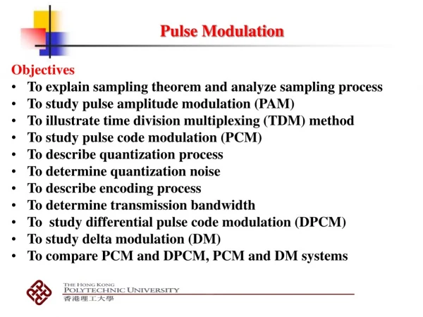
Chapter 11. Sampling and Pulse Modulation • The Sampling Theorem • PAM -- Natural and Flat-Top Sampling Time-Division Multiplexing (TDM) Intersymbol Interference (ISI) • Pulse Width and Pulse Position Modulation Demodulation • Digital Modulation Pulse Code Modulation (PCM) Delta Modulation (DM) • Qualitative Comparisons Of Pulse and Digital Modulation Systems
The Sampling Theorem Figure 11-1. Impulse sampling of an analog voltage.
The Sampling Theorem • A sampler is a mixer with a train of very narrow pulses as the local oscillator input. • If the analog input is sampled instantaneously at regular intervals at a rate that is at least twice the highest analog frequency fs> 2fa(max) • then the samples contain all of the information of the original signal.
The Sampling Theorem • The analog signal v(t) has a signal spectrum represented by the Fourier transform V(f), • and the sampling signal consists of instantaneous impulses every nTs sec, where n = 0, +1, +2, … • The Fourier transform of s(t) is
The Sampling Theorem • The time-domain product performed by the sampler produces a sampled output spectrum given by • where this spectrum consists of replicas of the analog signal spectrum V(f), translated in frequency by each of the sampling frequency harmonics.
The Sampling Theorem • The sampler is a wideband (harmonic) mixer producing upper and lower sidebands at each harmonic of the sampling frequency. • Figure 11-2a illustrates the correct way to sample: if sampling is done at fs > 2fA(max) the upper and lower sidebands do not overlap each other, • and the original information can be recovered by passing the signal through a low-pass filter (see Figure 11-2c and d).
The Sampling Theorem Figure 11-2. Sample spectra and their outputs. (a) fs > 2fA(max) Nyquist criteria met. (b) fs < 2fA(max) Frequency foldover of “aliasing” distortion occurs. (c) fs > 2fA(max) and recovery of original information with low-pass filter. (d) The original analog signal spectrum following recovery as in (c).
The Sampling Theorem • However, if the sampling rate is less than the Nyquist rate, fs < 2fA(max) the sidebands overlap, as shown in Figure 11-2b. • The result is frequency-folding or aliasing distortion, which makes it impossible to recover the original signal without distortion.
Pulse Amplitude Modulation – Natural and Flat-Top Sampling • The circuit of Figure 11-3 is used to illustrate pulse amplitude modulation (PAM). The FET is the switch used as a sampling gate. • When the FET is on, the analog voltage is shorted to ground; when off, the FET is essentially open, so that the analog signal sample appears at the output. • Op-amp 1 is a noninverting amplifier that isolates the analog input channel from the switching function.
Pulse Amplitude Modulation – Natural and Flat-Top Sampling Figure 11-3. Pulse amplitude modulator, natural sampling.
Pulse Amplitude Modulation – Natural and Flat-Top Sampling • Op-amp 2 is a high input-impedance voltage follower capable of driving low-impedance loads (high “fanout”). • The resistor R is used to limit the output current of op-amp 1 when the FET is “on” and provides a voltage division with rd of the FET. (rd, the drain-to-source resistance, is low but not zero)
Pulse Amplitude Modulation – Natural and Flat-Top Sampling • The most common technique for sampling voice in PCM systems is to a sample-and-hold circuit. • As seen in Figure 11-4, the instantaneous amplitude of the analog (voice) signal is held as a constant charge on a capacitor for the duration of the sampling period Ts. • This technique is useful for holding the sample constant while other processing is taking place, but it alters the frequency spectrum and introduces an error, called aperture error, resulting in an inability to recover exactly the original analog signal.
Pulse Amplitude Modulation – Natural and Flat-Top Sampling • The amount of error depends on how mach the analog changes during the holding time, called aperture time. • To estimate the maximum voltage error possible, determine the maximum slope of the analog signal and multiply it by the aperture time DT in Figure 11-4.
Pulse Amplitude Modulation – Natural and Flat-Top Sampling Figure 11-4. Sample-and-hold circuit and flat-top sampling.
Time-Division Multiplexing • In the three-channel multiplexed PAM system of Figure 11-6, each channel is filtered and sampled once per revolution (cycle) of the commutator. • Notice that the commutator is performing both the sampling and the multiplexing. • The commutator must operate at a rate that satisfies the sampling theorem for each channel. • Consequently, the channel of highest cutoff frequency determines the commutation rate for the system of Figure 11-6.
Time-Division Multiplexing Figure 11-6. Time-division multiplex of three information sources.
Time-Division Multiplexing • As an example, suppose the maximum signal frequency for the three input channels are fA1(max) = 4 kHz, fA2(max) = 20 kHz, and fA3(max) = 4 kHz. • For the TDM system of Figure 11-6, the multiplexing must proceed at f> 2fA(max) = 40 kHz to satisfy the worst-case condition.
Time-Division Multiplexing • We can calculate the transmission line pulse rate as follows: The commutator completes one cycle, called a frame, every 1/40 kHz = 25 ms. • Each time around, the commutator picks up a pulse from each of the three channels. Hence, there are 3 pulses/frame x 40k frames/s = 120k pulses/s.
Time-Division Multiplexing • The 4 kHz channel is being sampled at five times the rate required by the sampling theorem. But if we slow down the commutator, the 20-kHz channel will be inadequately sampled. • One the thought might be to multiplex at 8 k-frames/sec and sample the 20-kHz channel 5 times per frame. • If you sketch this, as is done in Figure 11-7, you discover that there are 7 pulses/frame x 8k frames/s = 56k pulses/s, which looks good.
Time-Division Multiplexing Figure 11-7. Possible TDM solution.
Time-Division Multiplexing • The two missing samples stolen from the 20-kHz channel results in inadequate sampling and periodic aliasing distortion. • For no errors, the commutation rate must be 17.14 kHz, producing 120k samples/s on the transmission line. • A better scheme is shown in Figure 11-8 with insertion of channel 1 and 3 between two samples of channel 2. • With 12.5 ms/pulse and 7 pulses/frame, the multiplexing rate can be (2 pulses/25ms)/(7 pulses/frame) = 11.428k frames/s and (11.428k frames/s) x (7 pulses/frame) = 80k pulses/s with no errors.
Time-Division Multiplexing Figure 11-8. TDM solution for minimum transmission line pulse rate.
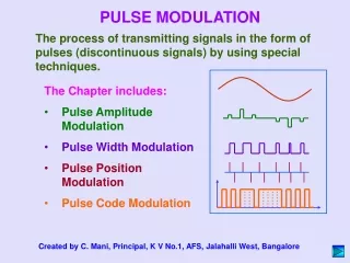
Pulse Width and Pulse Position Modulation • In pulse width modulation (PWM), the width of each pulse is made directly proportional to the amplitude of the information signal. • In pulse position modulation, constant-width pulses are used, and the position or time of occurrence of each pulse from some reference time is made directly proportional to the amplitude of the information signal. • PWM and PPM are compared and contrasted to PAM in Figure 11-11.
Pulse Width and Pulse Position Modulation Figure 11-11. Analog/pulse modulation signals.
Pulse Width and Pulse Position Modulation • Figure 11-12 shows a PWM modulator. This circuit is simply a high-gain comparator that is switched on and off by the sawtooth waveform derived from a very stable-frequency oscillator. • Notice that the output will go to +Vcc the instant the analog signal exceeds the sawtooth voltage. • The output will go to -Vcc the instant the analog signal is less than the sawtooth voltage. With this circuit the average value of both inputs should be nearly the same. • This is easily achieved with equal value resistors to ground. Also the +V and –V values should not exceed Vcc.
Pulse Width and Pulse Position Modulation Figure 11-12. Pulse width modulator.
Pulse Width and Pulse Position Modulation • A 710-type IC comparator can be used for positive-only output pulses that are also TTL compatible. PWM can also be produced by modulation of various voltage-controllable multivibrators. • One example is the popular 555 timer IC. Other (pulse output) VCOs, like the 566 and that of the 565 phase-locked loop IC, will produce PWM. • This points out the similarity of PWM to continuous analog FM. Indeed, PWM has the advantages of FM---constant amplitude and good noise immunity---and also its disadvantage---large bandwidth.
Demodulation • Since the width of each pulse in the PWM signal shown in Figure 11-13 is directly proportional to the amplitude of the modulating voltage. • The signal can be differentiated as shown in Figure 11-13 (to PPM in part a), then the positive pulses are used to start a ramp, and the negative clock pulses stop and reset the ramp. • This produces frequency-to-amplitude conversion (or equivalently, pulse width-to-amplitude conversion). • The variable-amplitude ramp pulses are then time-averaged (integrated) to recover the analog signal.
Pulse Width and Pulse Position Modulation Figure 11-13. Pulse position modulator.
Demodulation • As illustrated in Figure 11-14, a narrow clock pulse sets an RS flip-flop output high, and the next PPM pulses resets the output to zero. • The resulting signal, PWM, has an average voltage proportional to the time difference between the PPM pulses and the reference clock pulses. • Time-averaging (integration) of the output produces the analog variations. • PPM has the same disadvantage as continuous analog phase modulation: a coherent clock reference signal is necessary for demodulation. • The reference pulses can be transmitted along with the PPM signal.
Demodulation • This is achieved by full-wave rectifying the PPM pulses of Figure 11-13a, which has the effect of reversing the polarity of the negative (clock-rate) pulses. • Then an edge-triggered flipflop (J-K or D-type) can be used to accomplish the same function as the RS flip-flop of Figure 11-14, using the clock input. • The penalty is: more pulses/second will require greater bandwidth, and the pulse width limit the pulse deviations for a given pulse period.
Demodulation Figure 11-14. PPM demodulator.
Pulse Code Modulation (PCM) • Pulse code modulation (PCM) is produced by analog-to-digital conversion process. • As in the case of other pulse modulation techniques, the rate at which samples are taken and encoded must conform to the Nyquist sampling rate. • The sampling rate must be greater than, or equal to, twice the highest frequency in the analog signal, fs> 2fA(max)
Pulse Code Modulation (PCM) • A simple example to illustrate the pulse code modulation of an analog signal is shown in Figure 11-15. • Here, an analog input sample becomes three binary digits (bits) in a sequence which represents the amplitude of the analog sample. • At time t = 1, the analog signal is 3 V. This voltage is applied to the encoder for a time long enough that the three-bit digital "word", 011, is produced.
Pulse Code Modulation (PCM) • The second sample at t = 2 has an amplitude of 6 V, which is encoded as 110. • This particular example system is conveniently set up so that the analog value (decimal) is encoded with its binary equivalent.
Pulse Code Modulation (PCM) Figure 11-15. A 3-bit PCM system showing A/D conversion.
Delta Modulation (DM) • Like PCM, a delta modulation system consists of an encoder and a decoder; • unlike PCM, however, a delta modulator generates single-bit words that represent the difference (delta) between the actual input signal and a quantized approximation of the preceding input signal sample. • This is represented in Figure 11-19 with a sample-and-hold, comparator, up-down counter staircase generator, and a D-type flip-flop (D-FF) to derive the digital pulse stream.
Delta Modulation (DM) • The continuous analog signal is band-limited in the low-pass filter (LPF) to prevent aliasing distortion, as in any sampling system. • The analog signal VA is then compared to its discrete approximation VB.
Delta Modulation (DM) Figure 11-19. Possible delta modulation encoder.
Delta Modulation (DM) • Ifthe amplitude of VA is greater than VB , the comparator goes high, calling for positive going steps from the staircase generator. • if, however, VB exceeds VA, the comparator goes low, calling for negative-going from the staircase generator. • The comparator also sets the D flip-flop (D-FF) and the output will be properly clocked because the edge-triggered D-FF can change state only at rising edges of the input clock.
Delta Modulation (DM) • Decoding of the delta modulation (DM) signal can be accomplished with an up-down staircase generator and a smoothing filter • or simply by integrating the DM pulses as shown in Figure 11-20. The resulting demodulated signal is illustrated as curve B. • A practical implementation of a delta modulator is shown in Figure 11-21, where the up-down counter and digital-to-analog converter (DAC) comprise the staircase generator of Figure 11-19. • The delta modulator of Figure 11-21 is usually referred to as a tracking or servo analog-to-digital converter.
Delta Modulation (DM) Figure 11-20. DM demodulator.
Delta Modulation (DM) Fig. 11-21. Up-down staircase generator for delta modulator.
Delta Modulation (DM) • As seen in Figure 11-22, the critical parameters determining the quality of a system using a constant step size are the designer’s choice of step size and sampling period length • With too small a step size, the analog signal changes cannot be followed closely enough; this is called slope overload (Figure 11-22a). • With too large a step size, two problems arise: poor signal approximation (resolution) and large quantization noise (Figure 11-22b). This condition is called granular noise.
Delta Modulation (DM) • Too long a period has the same problem as too small a step size and poor resolution (Figure 11-22c). • When the period is too short, too much transmission bandwidth is required. Fig. 11-22. Critical design parameters in constant step-size linear delta modulation.
Delta Modulation (DM) Example: • A 5-V pk, 4-kHz sinusoid is to be converted to a digital signal by delta modulation. The step size must be 10 mV. • Determine the minimum clock rate that will allow the DM system to follow exactly the fastest input analog signal change, that is, to avoid slope overload.
Delta Modulation (DM) Solution: • The fastest rate of change of a sinewave, v(t) = Vsinwt is the slope at the zero crossover points (t = 0 in Figure 11-23). slope = dv(t)/dt = (d/dt).(Vsinwt) = wVcoswt. • At t = 0, the slope iswV.cos0 = wVor Dv/Dt = 2pfV,where f is the frequency of the analog sinusoid.
Delta Modulation (DM) • Dt is half the clock period because steps occur only at positive transitions of the clock in a practical system. • Thus, Tclock = 2Dt = 1/fclock, so that fclock = 1/2Dt = 1/(2x0.079x10-6 s/cycle) = 6.3 MHz. Figure 11-23. Example problem.
Practical DM • A circuit configuration in present use for telecom-munication applications involving filters, speech scramblers, instrumentation, and remote motor control is shown in Figure 11-24. • To demodulate the digital signal simple integrate the pulses. In fact, the integrator has the same RC time constant as the modulator above. • The integrated demodulator output is the same as the B curve of Fig. 11-24. The integrator output is then put through a sharp cutoff LPF to smooth out the final gain amplifier (VGA) and decision logic as indicated in Fig. 11-25 for adaptive DM.
Practical DM Fig. 11-24. Integrating linear delta modulator block diagram and signals.