MERGE – Presentation to EMF 21
160 likes | 328 Vues
MERGE – Presentation to EMF 21. Alan S. Manne, Stanford University Richard G. Richels, EPRI. Stanford University December 2003. Features of MERGE . Intertemporal computable general equilibrium model Perfect foresight 9 regions Time periods: decades from 2000 through 2150

MERGE – Presentation to EMF 21
E N D
Presentation Transcript
MERGE – Presentation toEMF 21 Alan S. Manne, Stanford University Richard G. Richels, EPRI Stanford University December 2003
Features of MERGE Intertemporal computable general equilibrium model Perfect foresight 9 regions Time periods: decades from 2000 through 2150 Bottom-up model of energy supplies; top-down model of electric and nonelectric energy demands Tradeables: oil, gas, carbon emission rights Technical progress: both learn-by-doing and exogenous Three greenhouse gases: co2, ch4 and n2o Tradeoffs between gases based on “efficiency” prices rather than gwp Website: www.stanford.edu/group/MERGE
Features Added Specifically for EMF 21 Second basket of gases: short- and long-lived f-gases (slf, llf) Baseline emissions of four non-co2 gases from EPA through 2020 Extrapolated emissions growth: linear at rates projected between 2000 and 2020 Marginal abatement cost curves of four non-co2 gases from EPA Extrapolated technical progress Carbon sinks – afforestation - cumulative quantities as well as annual growth and decline limits Reported the five long-term scenarios requested by EMF; mostly global rather than regional results
Marginal Costs of Abatement – Technical Progress Multipliers for all Gases but CO2 $/tce 2010 2050 2100
Global Radiative Forcing Percentages2000-2100 - reference case slf 2% llf ~0% n2o 15% ch4 8% co2 75%
Control Cases • In reference case, temperature increases by 3.2 degrees C between 2000 and 2100. • Alternatively, limit the radiative forcing increase to 4.5 watts/square meter. Between 2000 and 2100, this leads to a temperature increase of about 2.5 degrees C. • Limit temperature increase to 0.2 degrees C per decade from 2020 onward. This leads to an extremely high value for carbon emission rights during the early decades. • Compare two abatement cases: energy-related CO2 only vs. all greenhouse gases plus afforestation.
Ratio of Efficiency Prices to GWP’s ( 4.5 watts/square meter – multigas )