Understanding Graphics Pipeline: Visibility Techniques and Surface Rendering Methods
220 likes | 368 Vues
This document explores crucial concepts in the graphics pipeline, focusing on visibility techniques such as back-face culling, Painter’s Algorithm, and depth sorting. It explains how simple primitives can be converted to pixels, identifies which parts should be visible, and discusses potential issues with overlapping surfaces and order ambiguity. Methods like Binary Space Partitioning (BSP) and Z-buffering are highlighted, with algorithms for building trees and displaying polygons. Practical implications regarding memory usage and implementation ease are also considered.

Understanding Graphics Pipeline: Visibility Techniques and Surface Rendering Methods
E N D
Presentation Transcript
Graphics PipelineHidden Surfaces CMSC 435/634
Visibility • We can convert simple primitives to pixels • Which primitives (or parts of primitives) should be visible?
Back-face Culling • Polygon is back-facing if VN > 0 • Assuming view is along –Z V = (0,0,1) VN = 0 + 0 + Nz • Simplifying further • If Nz≤ 0, then cull • Works for non-overlapping convex polyhedra • With concave polyhedra, some hidden surfaces will not be culled
Painter’s Algorithm • First polygon: • (6,3,10), (11, 5,10), (2,2,10) • Second polygon: • (1,2,8), (12,2,8), (12,6,8), (1,6,8) • Third polygon: • (6,5,5), (14,5,5), (14,10,5),( 6,10,5)
Painter’s Algorithm • Given List of polygons Array of colors: color[x,y] • Algorithm Sort polygons on minimum z For each polygon P in sorted list For each pixel (x,y,z) in P color[x,y] = color(P,x,y)
Painter’s Algorithm: Cycles • Which to scan first? • Split along line, then scan 1,2,3,4 (or split another polygon and scan accordingly) • Moral: Painter’s algorithm is fast and easy, except for detecting and splitting cycles and other ambiguities
Depth-sort: Overlapping Surfaces • Assume you have sorted by maximum Z • Then if Zmin > Z’max, the surfaces do not overlap each other (minimax test) • Correct order of overlapping surfaces may be ambiguous. Check it.
Depth-sort: Overlapping Surfaces • No problem: paint S, then S’ • Problem: painting in either order gives incorrect result • Problem? Naïve order S S’ S”; correct order S’ S” S
Depth-sort: Order Ambiguity • Bounding rectangles in xy plane do not overlap • Check overlap in x x’min > xmax or xmin > x’max -> no overlap • Check overlap in y y’min > ymax or ymin > y’max -> no overlap • Surface S is completely behind S’ relative to viewing direction. • Substitute all vertices of S into plane equation for S’ • if all are “inside”(< 0), no ambiguity
Depth-sort: Order Ambiguity 3. Surface S’ is completely in front S relative to viewing direction. • Substitute all vertices of S’ into plane equation for S • if all are “outside” ( >0), no ambiguity
Building a BSP Tree • Use pgon3 as root, split on its plane • Pgon 5 split into 5a and 5b
Building a BSP Tree • Split left subtree at pgon 2
Building a BSP Tree • Split right subtree at pgon 4
Building a BSP Tree • Alternate tree if splits are made at 5, 4, 3, 1
BSP Tree: Building the Tree BSPTreeMakeBSP ( Polygon list ) if ( list is empty ) return null else { root = some polygon ; remove it from the list backlist = frontlist = null for ( each remaining polygon in the list ) if ( p in front of root ) addToList( p, frontlist ) else if ( p in back of root ) addToList( p, backlist ) else splitPolygon(p,root,frontpart,backpart) addToList( frontpart, frontlist ) addToList( backpart, backlist ) return (combineTree(MakeBSP(frontlist), root, MakeBSP(backlist)))
BSP Tree: Displaying the Tree DisplayBSP ( tree ) if ( tree not empty ) if ( viewer in front of root ) DisplayBSP( tree -> back ) DisplayPolygon( tree -> root ) DisplayBSP( tree -> front ) else DisplayBSP( tree -> front ) DisplayPolygon( tree -> root ) DisplayBSP( tree -> back )
BSP Tree Display • Built BSP tree structure
BSP Tree Display C in front of 3 (order back/front) draw 4/5b branch C in back of 4 (order front/back) nothing in front of 4 draw 4 draw 5b draw 3 draw 1/2/5a branch C in back of 2 (order front/back) draw 5a draw 2 draw 1
Z-Buffer • First polygon • (1, 1, 5), (7, 7, 5), (1, 7, 5) • scan it in with depth • Second polygon • (3, 5, 9), (10, 5, 9), (10, 9, 9), (3, 9, 9) • Third polygon • (2, 6, 3), (2, 3, 8), (7, 3, 3)
Z-Buffer Algorithm • Originally by Cook, Carpenter, Catmull • Given List of Polygons Array of depths: zbuffer[x,y] initialized to ∞ Array of colors: color[x,y] • Algorithm For each Polygon P For each pixel (x,y,z) in P If z < zbuffer[x,y] zbuffer[x,y] = z color[x,y] = color(P,x,y)
Z-Buffer Characteristics • Good • Easy to implement • Requires no sorting of surfaces • Easy to put in hardware • Bad • Requires lots of memory (about 9MB for 1280x1024 display) • Can alias badly (only one sample per pixel) • Cannot handle transparent surfaces