Graphics Pipeline Hidden Surface
Graphics Pipeline Hidden Surface. CMSC 435/634. Visibility. We can convert simple primitives to pixels/fragments How do we know which primitives (or which parts of primitives) should be visible?. Back-face Culling. Polygon is back-facing if V N > 0 Assuming view is along Z (V=0,0,1)


Graphics Pipeline Hidden Surface
E N D
Presentation Transcript
Graphics PipelineHidden Surface CMSC 435/634
Visibility • We can convert simple primitives to pixels/fragments • How do we know which primitives (or which parts of primitives) should be visible?
Back-face Culling • Polygon is back-facing if • VN > 0 • Assuming view is along Z (V=0,0,1) • VN = (0 + 0 + zn) • Simplifying further • If zn> 0, then cull • Works for non-overlapping convex polyhedra • With concave polyhedra, some hidden surfaces will not be culled
Painter’s Algorithm • First polygon: • (6,3,10), (11, 5,10), (2,2,10) • Second polygon: • (1,2,8), (12,2,8), (12,6,8), (1,6,8) • Third polygon: • (6,5,5), (14,5,5), (14,10,5),( 6,10,5)
Painter’s Algorithm • Given List of polygons {P1, P2, …. Pn) An array of Intensity [x,y] • Begin Sort polygon list on minimum Z (largest z-value comes first in sorted list) For each polygon P in selected list do For each pixel (x,y) that intersects P do Intensity[x,y] = intensity of P at (x,y) Display Intensity array
Painter’s Algorithm: Cycles • Which order to scan? • Split along line, then scan 1,2,3
Painter’s Algorithm: Cycles • Which to scan first? • Split along line, then scan 1,2,3,4 (or split another polygon and scan accordingly) • Moral: Painter’s algorithm is fast and easy, except for detecting and splitting cycles and other ambiguities
Depth-sort: Overlapping Surfaces • Assume you have sorted by maximum Z • Then if Zmin > Z’max, the surfaces do not overlap each other (minimax test) • Correct order of overlapping surfaces may be ambiguous. Check it.
Depth-sort: Overlapping Surfaces • No problem: paint S, then S’ • Problem: painting in either order gives incorrect result • Problem? Naïve order S S’ S”; correct order S’ S” S
Depth-sort: Order Ambiguity • Bounding rectangles in xy plane do not overlap • Check overlap in x x’min > xmax or xmin > x’max -> no overlap • Check overlap in y y’min > ymax or ymin > y’max -> no overlap • Surface S is completely behind S’ relative to viewing direction. • Substitute all vertices of S into plane equation for S’, if all are “inside” ( < 0), then there is no ambiguity
Depth-sort: Order Ambiguity 3. Surface S’ is completely in front S relative to viewing direction. • Substitute all vertices of S’ into plane equation for S, if all are “outside” ( >0), then there is no ambiguity
Building a BSP Tree • Use pgon 3 as root, split on its plane • Pgon 5 split into 5a and 5b
Building a BSP Tree • Split left subtree at pgon 2
Building a BSP Tree • Split right subtree at pgon 4
Building a BSP Tree • Alternate tree if splits are made at 5, 4, 3, 1
BSP Tree: Building the Tree BSPTree MakeBSP ( Polygon list ) { if ( list is empty ) return null else { root = some polygon ; remove it from the list backlist = frontlist = null for ( each remaining polygon in the list ) { if ( p in front of root ) addToList ( p, frontlist ) else if ( p in back of root ) addToList ( p, backlist ) else { splitPolygon (p,root,frontpart,backpart) addToList ( frontpart, frontlist ) addToList ( backpart, backlist ) } } return (combineTree(MakeBSP(frontlist),root, MakeBSP(backlist))) } }
BSP Tree: Displaying the Tree DisplayBSP ( tree ) { if ( tree not empty ) { if ( viewer in front of root ) { DisplayBSP ( tree -> back ) DisplayPolygon ( tree -> root ) DisplayBSP ( tree -> front ) } else { DisplayBSP ( tree -> front ) DisplayPolygon ( tree -> root ) DisplayBSP ( tree -> back ) } } }
BSP Tree Display • Built BSP tree structure
BSP Tree Display C in front of 3
BSP Tree Display C in front of 3 (<3) C behind 4 (>4) none
BSP Tree Display C in front of 3 (<3) C behind 4 (>4) none (=4) display 4
BSP Tree Display C in front of 3 (<3) C behind 4 (>4) none (=4) display 4 (<4) display 5b
BSP Tree Display C in front of 3 (<3) C behind 4 (>4) none (=4) display 4 (<4) display 5b (=3) display 3
BSP Tree Display C in front of 3 (<3) C behind 4 (>4) none (=4) display 4 (<4) display 5b (=3) display 3 (>3) C behind 2
BSP Tree Display C in front of 3 (<3) C behind 4 (>4) none (=4) display 4 (<4) display 5b (=3) display 3 (>3) C behind 2 (>2) display 5a
BSP Tree Display C in front of 3 (<3) C behind 4 (>4) none (=4) display 4 (<4) display 5b (=3) display 3 (>3) C behind 2 (>2) display 5a (=2) display 2
BSP Tree Display C in front of 3 (<3) C behind 4 (>4) none (=4) display 4 (<4) display 5b (=3) display 3 (>3) C behind 2 (>2) display 5a (=2) display 2 (<2) display 1
Scanline Algorithm • Simply problem by considering only one scanline at a time • intersection of 3D scene with plane through scanline
Scanline Algorithm • Consider xz slice • Calculate where visibility can change • Decide visibility in each span
Scanline Algorithm • Sort polygons into sorted surface table (SST) based on first Y • Initialize y and active surface table (AST) Y = first nonempty scanline AST = SST[y] • Repeat until AST and SST are empty Identify spans for this scanline (sorted on x) For each span determine visible element (based on z) fill pixel intensities with values from element Update AST remove exhausted polygons y++ update x intercepts resort AST on x add entering polygons • Display Intensity array
Scanline Visibility Algorithm • Scanline • AST: ABC • Spans • 0 -> x1 • x1 -> x2 • x2 -> max background ABC background
Scanline Visibility Algorithm • Scanline • AST: ABCDEF • Spans • 0 -> x1 • x1 -> x2 • x2 -> x3 • x3 -> x4 • x4-> max background ABC background DEF background
Scanline Visibility Algorithm • Scanline • AST: ABCDEF • Spans • 0 -> x1 • x1 -> x2 • x2 -> x3 • x3 -> x4 • x4-> max background ABC DEF DEF background
Scanline Visibility Algorithm • Scanline + 1 • Spans • 0 -> x1 • x1 -> x2 • x2 -> x3 • x3 -> x4 • x4-> max background ABC DEF DEF background • Scanline + 2 • Spans • 0 -> x1 • x1 -> x2 • x2 -> x3 • x3 -> x4 • x4-> max background ABC background DEF background
Characteristics of Scanline Algorithm • Good • Little memory required • Can generate scanlines as required • Can antialias within scanline • Fast • Simplification of problem simplifies geometry • Can exploit coherence • Bad • Fairly complicated to implement • Difficult to antialias between scanlines
Z-Buffer • First polygon • (1, 1, 5), (7, 7, 5), (1, 7, 5) • scan it in with depth • Second polygon • (3, 5, 9), (10, 5, 9), (10, 9, 9), (3, 9, 9) • Third polygon • (2, 6, 3), (2, 3, 8), (7, 3, 3)
Z-Buffer Algorithm • Originally Cook, Carpenter, Catmull • Given List of polygons {P1, P2, …., Pn} An array z-buffer[x,y] initialized to +infinity An array Intensity[x,y] • Begin For each polygon P in selected list do For each pixel (x,y) that intersects P do Calculate z-depth of P at (x,y) If z-depth < z-buffer[x,y] then Intensity[x,y] = intensity of P at (x,y) Z-buffer[x,y] = z-depth Display Intensity array
Z-Buffer Characteristics • Good • Easy to implement • Requires no sorting of surfaces • Easy to put in hardware • Bad • Requires lots of memory (about 9MB for 1280x1024 display) • Can alias badly (only one sample per pixel) • Cannot handle transparent surfaces
A-Buffer Method • Basically z-buffer with additional memory to consider contribution of multiple surfaces to a pixel • Need to store • Color (rgb triple) • Opacity • Depth • Percent area covered • Surface ID • Misc rendering parameters • Pointer to next
Taxonomy of Visibility Algorithms • Ivan Sutherland -- A Characterization of Ten Hidden Surface Algorithms • Basic design choices • Space for operations • Object • Image • Object space • Loop over objects • Decide the visibility of each • Timing of object sort • Sort-first • Sort-last
Taxonomy of Visibility Algorithms • Image space • Loop over pixels • Decide what’s visible at each • Timing of sort at pixel • Sort first • Sort last • Subdivide to simplify
Taxonomy Revisted • Another dimension • Point-sampling • continuous