Hidden surface removal

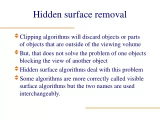
1. Hidden surface removal • Clipping algorithms will discard objects or parts of objects that are outside of the viewing volume • But, that does not solve the problem of one objects blocking the view of another object • Hidden surface algorithms deal with this problem • Some algorithms are more correctly called visible surface algorithms but the two names are used interchangeably. Lecture 9

2. Visibility of primitives • We don’t want to waste time rendering primitives which don’t contribute to the final image. • A scene primitive can be invisible for 3 reasons: • Primitive lies outside field of view • Primitive is back-facing (under certain conditions) • Primitive is occluded by one or more objects nearer the viewer • How do we remove these efficiently? • How do we identify these efficiently? Lecture 9

3. The visibility problem. Removal of faces facing away from the viewer. Removal of faces obscured by closer objects. Lecture 9

4. Visible surface algorithms. Hidden/Visible Surface/Line Elimination/Determination • Requirements • Handle diverse set of geometric primitives • Handle large number of geometric primitives Classification: Sutherland, Sproull, Schumacher (1974): • Object Space • Geometric calculations involving polygons • Floating point precision: Exact • Often process scene in object order • Image Space • Visibility at pixel samples • Integer precision • Often process scene in image order Lecture 9

5. Visible surface algorithms. Object based methods • Consider objects pairwise at a time, do it iteratively, comparing each polygon with the rest of polygons: • A and B both completely visible – display both • A completely obscure B – display only A (vice versa) • A and B partially obscure each other – calculate visible parts of each polygon • Complexity is O(k2) – regard the determination of which case it is and any required calculation of visible parts of each polygon as a single operation Image based methods • per pixel, consider a ray that leaves the center of projection and passes through a pixel and decide which object should appear at the pixel and what colour/light/texture it should be drawn in Lecture 9

6. Back face culling. • We saw in modelling, that the vertices of polyhedra are oriented in an anticlockwise manner when viewed from outside – surface normal N points out. • Project a polygon. • Test z component of surface normal. If negative – cull, since normal points away from viewer. • Or if N.V > 0 we are viewing the back face so polygon is obscured (A polygon faces away from the viewer if the angle between the surface normal (N) and the viewing direction (V) is less than 90 degrees V.N > 0) • Only works for convex objects without holes, ie. closed orientable manifolds. Lecture 9

7. Back face culling • Back face culling can be applied anywhere in the pipeline: world or camera coords, NDC (normalised device co-ordinate), image space. • Where is the best point? What portion of the scene is eliminated, on average? • Depends on application • If we clip our scene to the view frustrum, then remove all back-facing polygons – are we done? • NO! Most views involve overlapping polygons. Lecture 9

8. How de we handle overlapping? How about drawing the polygons in the “right order” so that we get the correct result ( eg. blue, then green, then peach)? Is it just a sorting problem ? Yes it is for 2D, but in 3D we can encounter intersecting polygons or groups of non-intersecting polygons which form a cycle where order is impossible (later). Lecture 9

9. Z-buffer Algorithm • Some polygons will be obscured by others - we only want to draw the visible polygons • Suppose polygons have been passed through the projection transformation, with the z coordinate retained (ie the depth information) - suppose z normalized to range 0 to 1 • For each pixel (x,y), we want to draw the polygon nearest to the camera, ie largest z y x z camera Lecture 9

10. Z-buffer Algorithm • We require two buffers: • frame buffer to hold colour of each pixel • z-buffer to hold depth information for each pixel • Initialize all depth(x,y) to 0 and refresh(x,y) to background colour • For each pixel compare depth value z to current depth(x,y) • if z > depth(x,y) then • depth(x,y)=z • Frame buffer (x,y) = Isurface(x,y) (gouraud/phong shading) A B y z2 z1 x z Lecture 9

11. Z-buffer Algorithm Fill each pixel with background and set each z  colour to infinity  For each polygonP in the scene Do  For each pixel (x,y) in P's projection Do calculate z-coordinate, zp of p at (x,y)  IF zp < value in Z-buffer at ( x,y ) THEN replace value in Z-buffer at (x,y) by Zp colour pixel (x,y) in colour of p  End IF  End For  End For Lecture 9

12. Determining depth. • Only one subtraction needed • Depth coherence. Lecture 9

13. Z Buffer - Strengths and Weaknesses Advantage • Simple to implement in hardware. • Add additional z interpolator for each primitive. • Memory for z-buffer is now not expensive • Diversity of primitives – not just polygons. • Unlimited scene complexity • Don’t need to calculate object-object intersections. Disadvantage • Extra memory and bandwidth • Waste time drawing hidden objects • Limited precision for depth calculations in complex scenes can be a problem Lecture 9

14. Z-compositing Colour photograph. Can use depth other than from polygons. Laser range return. Reflected laser power Data courtesy of UNC. Lecture 9

15. Ray casting. • Sometimes referred to as Ray-tracing. • Involves projecting an imaginary ray from the centre of projection (the viewers eye) through the centre of each pixel into the scene. Scene Eyepoint Window Lecture 9

16. Computing ray-object intersections. • The heart of ray tracing. • e.g. sphere ( the easiest ! ). • Expand, substitute for x,y & z. • Gather terms in t. • Quadratic equation in t. Solve for t. • No roots – ray doesn’t intersect. • 1 root – ray grazes surface. • 2 roots – ray intersects sphere, • (entry and exit) Lecture 9

17. Ray-polygon intersection. • Not so easy ! • Determine whether ray intersects polygon’s plane. • Determine whether intersection lies within polygon. • Easiest to determine (2) with an orthographic projection onto the nearest axis and the 2D point-in-polygon test. z Ray x y Lecture 9

18. Ray casting. • Easy to implement for a variety of primitives – only need a ray-object intersection function. • Pixel adopts colour of nearest intersection. • Can draw curves and surfaces exactly – not just triangles ! • Can generate new rays inside the scene to correctly handle visibility with reflections, refraction etc – recursive ray-tracing. • Can be extended to handle global illumination. • Can perform area-sampling using ray super-sampling. • But… too expensive for real-time applications. Lecture 9

19. Examples of Ray-traced images. Lecture 9

20. Depth Sort Methods • The Depth Sort Algorithm initially sorts the faces in the object into back to front order. • The faces are then scan converted in this order onto the screen. • Thus a face near the front will obscure a face at the back by overwriting it at any points where their projections overlap. • This accomplishes hidden-surface removal without any complex intersection calculations between the two projected faces. This latter technique of painting the object in back to front order is often called The Painter's Algorithm • The Depth Sort algorithm is a hybrid algorithm in that it sorts in object space and does the final rendering in image space. Lecture 9

21. A B z x Depth Sort Methods • The basic algorithm : • Sort all polygons in descending order of maximum z-values. • Resolve any ambiguities in this ordering. • Scan convert each polygon in the order generated by steps (1) and (2). • The necessity for step (2) can be seen in the simple case: A precedes B in order of maximum z but B should precede A in writing order. • At step (2) the ordering produced by (1) must be confirmed. This is done by making more precise comparisons between polygons whose z-extents overlap Lecture 9

22. BSP (Binary Space Partitioning) Tree. • One of class of “list-priority” algorithms – returns ordered list of polygon fragments for specified view point (static pre-processing stage). • Choose polygon arbitrarily • Divide scene into front (relative to normal) and back half-spaces. • Split any polygon lying on both sides. • Choose a polygon from each side – split scene again. • Recursively divide each side until each node contains only 1 polygon. 5 2 3 1 4 View of scene from above Lecture 9

23. 5 5a 5b 2 3 1 4 3 back front 1 2 5a 4 5b BSP Tree. • Choose polygon arbitrarily • Divide scene into front (relative to normal) and back half-spaces. • Split any polygon lying on both sides. • Choose a polygon from each side – split scene again. • Recursively divide each side until each node contains only 1 polygon. Lecture 9

24. BSP Tree. 5 5a 5b 2 • Choose polygon arbitrarily • Divide scene into front (relative to normal) and back half-spaces. • Split any polygon lying on both sides. • Choose a polygon from each side – split scene again. • Recursively divide each side until each node contains only 1 polygon. 3 1 4 3 back front 2 4 5b front 5a 1 Lecture 9

25. 5 5a 5b 2 3 1 4 3 back front 2 4 front 5a 1 5b BSP Tree. • Choose polygon arbitrarily • Divide scene into front (relative to normal) and back half-spaces. • Split any polygon lying on both sides. • Choose a polygon from each side – split scene again. • Recursively divide each side until each node contains only 1 polygon. Lecture 9

26. BSP Tree. 5 2 • Choose polygon arbitrarily • Divide scene into front (relative to normal) and back half-spaces. • Split any polygon lying on both sides. • Choose a polygon from each side – split scene again. • Recursively divide each side until each node contains only 1 polygon. 3 1 4 5 back 4 back Alternate formulation starting at 5 3 front 1 back 2 Lecture 9

27. Displaying a BSP tree. • Once we have the regions – need priority list • BSP tree can be traversed to yield a correct priority list for an arbitrary viewpoint. • Start at root polygon. • If viewer is in front half-space, draw polygons behind root first, then the root polygon, then polygons in front. • If polygon is on edge – either can be used. • Recursively descend the tree. • If eye is in rear half-space for a polygon – then can back face cull. Lecture 9

28. BSP Tree. • A lot of computation required at start. • Try to split polygons along good dividing plane • Intersecting polygon splitting may be costly • Cheap to check visibility once tree is set up. • Can be used to generate correct visibility for arbitrary views.  Efficient when objects don’t change very often in the scene. Lecture 9

29. Warnock’s Algorithm • Elegant hybrid of object-space and image-space. • Uses standard graphics solution:- if situation too complex then subdivide problem. • Start with root window: • If zero or one intersecting, contained or surrounding polygon then scan convert window • Else subdivide window as quadtree • Recurse until zero or one polygon, or some set depth • Depth may be pixel resolution, display nearest polygon Lecture 9

30. Warnock’s example Lecture 9

31. Warnock performance measure • Warnock’s algorithm: • Screen-space subdivision (screen resolution, r = w*h) hybrid object-space & image-space algorithm good for relatively few static primitives, precise. • Working set size (memory requirement): O(n) • Storage overhead (over & above model): O(n lg r) • Time to resolve visibility to screen precision: O(n*r) • Overdraw (depth complexity – how often a typical pixel is written by rasterization process): none Lecture 9