Real-time Mesh Simplification Using the GPU
Real-time Mesh Simplification Using the GPU. Christopher DeCoro Natasha Tatarchuk 3D Application Research Group. Introduction. Implement Mesh Decimation in real-time Utilizes new Geometry Shader stage of GPU Achieves a 20x speedup over CPU . Project Motivation.


Real-time Mesh Simplification Using the GPU
E N D
Presentation Transcript
Real-time Mesh Simplification Using the GPU Christopher DeCoro Natasha Tatarchuk 3D Application Research Group
Introduction • Implement Mesh Decimation in real-time • Utilizes new Geometry Shader stage of GPU • Achieves a 20x speedup over CPU
Project Motivation • Massive Increases in submitted geometry • Geometry rendered per shadow map (6x for cubemap!) • Not always needed at highest resolution • Geometry not always known at build-time • Dynamically-skinned objects only finalized at run-time • May be customized to users machine based on capabilities, would need to be adapted at program load time • Could be dynamically generated per level, need to be adapted at level load time • Simplification therefore needs to be fast (or even real-time) Also, just as importantly… • We want applications that exercise & stress GS/GPU • Evaluate new capabilities of the GPU • Learn how to adapt previously CPU-bound algorithms • Develop GPU-centric methodologies • Identify future feature set for GS/GPU as a whole • Limitations still exist – which should be addressed?
Contributions • Mapping of Decimation to GPU • 20x speedup vs. CPU • Enables load-time or real-time usage • Detail Preservation by Non-linear Warping • Also applicable to CPU out-of-core decimation • General-purpose GPU Octree • Adaptive decimation w/ constant memory • Applications not limited to simplification: collision detection, frustum culling, etc.
Outline • Project Introduction and Motivation • Background • Decimation with Vertex Clustering • Geometry Shaders in Direct3D 10 • Geometry Shader-based Vertex Clustering • Adaptive Simplification w/ Non-linear Warps • Probabalistic Octrees on the GPU
Vertex Clustering • Reduces mesh resolution • High-res mesh as input • Low-res as output • All implemented on the GPU • Ideal for processing streamed out data • Useful when rendering multiple times (i.e. shadows) • Can handle enormous models from scanned data • Based on “Out-of-Core Simplification of Large Polygonal Models,” P. Lindstrom, 2000 Figure from [Lindstrom 2000]
Previous Rendering Pipeline • Vertex Shaders and Pixel Shaders • Limits 1 output per 1 input • No culling of triangles for decimation • Fixed destination for each stage • Result meshes cannot be (easily) saved and reused
DirectX10 Rendering Pipeline • Geometry Shader in between VS & PS • Called for each primitive (usually triangle) • Able to access all vertices of a primitive • Can compute per-face quantities • Breaks 1:1 input-output limitation • Allows triangles to be culled from pipeline • Allows stream-out of processed geometry • Decimated meshes can easily be saved and reused
Outline • Project Introduction and Motivation • Background • Geometry Shader-based Vertex Clustering • Overview • Quadric Generation • Optimal Position Computation • Final Clustering • Adaptive Simplification w/ Non-linear Warps • Probabilistic Octrees on the GPU
Algorithm Overview • Start with the input mesh • Shown divided into clusters • Pass 1: Compute the quadric map from mesh • Use GS to compute quadric • Accumulate in cluster map, an RT used as large array • Pass 2: For each cluster, compute optimal position • Solves a linear system given by quadrics • Pass 3: Collapse each vertex to representative • 9x9x9 grid shown Model Courtesy of Stanford Graphics Lab
Vertex Clustering Pipeline • Pass 1: Create Quadric Map • Input: Original Mesh • Computation: • Determine plane equation, face quadrics for triangle • Compute the cluster and address of each vertex • Pack quadric into RT at appropriate address • Output: Render Targets representing clusters with packed quadrics and average positions
Quadric Map Implementation //Map a point to its location in the cluster map array float2 writeAddr( float3 vPos ) { uint iX = clusterId(vPos) / iClusterMapSize.x; uint iY = clusterId(vPos) % iClusterMapSize.y; return expand( float2(iX,iY)/float(iClusterMapSize.x) ) + 1.0/iClusterMapSize.x; } [maxvertexcount(3)] void main( triangle ClipVertex input[3], inoutPointStream<FragmentData> stream ) { //For the current triangle, compute the area and normal float3 vNormal = (cross( input[1].vWorldPos - input[0].vWorldPos, input[2].vWorldPos - input[0].vWorldPos )); float fArea = length(vNormal)/6; vNormal = normalize(vNormal); //Then compute the distance of plane to the origin along the normal float fDist = -dot(vNormal, input[0].vWorldPos); //Compute the components of the face quadrics using the plane coefficients float3x3 qA = fArea*outer(vNormal, vNormal); float3 qb = fArea*vNormal*fDist; float qc = fArea*fDist*fDist; //Loop over each vertex in input triangle primitive for(int i=0; i<3; i++) { //Assign the output position in the quadric map FragmentData output; output.vPos = float4(writeAddress(input[i].vPos),0,1); //Write the quadric to be accumulated in the quadric map packQuadric( qA, qb, qc, output ); stream.Append( output ); } } • Start with the input mesh • Shown divided into clusters • Compute the quadric map from mesh • Use GS to compute quadric • Accumulate in cluster map, an RT used as large array • For each cluster, compute optimal position • Collapse each vertex to representative • 9x9x9 grid shown
Vertex Clustering Pipeline • Pass 2: Find Optimal Positions • Input: Cluster Map Render Targets, Full-screen Quad • Computation: • Determine if we can solve for optimal position • If not, fall back to vertex average • Output: Render Targets representing clusters with optimal position of representative vtx.
Optimal Positions Original Mesh • For each cell, need representative • Naïve solution: Use averages • Looks very blocky • Does not consider the original faces, only vertices • Implemented solution: Use quadrics • Quadrics are a measure of surface • We can solve for optimal position Simplified w/ Averages Simplified w/ Quadrics
Optimal Positions Implementation float3 optimalPosition(float2 vTexcoord) { float3 vPos = float3(0,0,0); float4 dataWorld, dataA0, dataB, dataA1; //Read the vertex average from the cluster map dataWorld = tClusterMap0.SampleLevel( sClusterMap0, vTexcoord, 0 ); int iCount = dataWorld.w; //Only compute optimal position if there are vertices in this cluster if( iCount != 0 ) { //Read all the data from the clustermap to reconstruct the quadric dataA0 = tClusterMap1.SampleLevel( sClusterMap1, vTexcoord, 0 ); dataA1 = tClusterMap2.SampleLevel( sClusterMap2, vTexcoord, 0 ); dataB = tClusterMap3.SampleLevel( sClusterMap3, vTexcoord, 0 ); //Then reassemble the quadric float3x3 qA = { dataA0.x, dataA0.y, dataA0.z, dataA0.y, dataA0.w, dataA1.x, dataA0.z, dataA1.x, dataA1.y }; float3 qB = dataB.xyz; float qC = dataA1.z; //Determine if inverting A is stable, if so, compute optimal position //If not, default to using the average position constfloat SINGULAR_THRESHOLD = 1e-11; if(determinant(quadricA) > SINGULAR_THRESHOLD ) vPos = -mul( inverse(quadricA), quadricB ); else vPos = dataWorld.xyz / dataWorld.w; } return vPos; } • Start with the input mesh • Shown divided into clusters • Compute the quadric map from mesh • Use GS to compute quadric • Accumulate in cluster map, an RT used as large array • For each cluster, compute optimal position • Collapse each vertex to representative • 9x9x9 grid shown
Vertex Clustering Pipeline • Pass 3: Decimate Mesh • Input: Cluster Map Render Targets, Input Mesh • Computation: • Find clusters, Remap vertices to representative • Determine if triangle becomes degenerate • If not, stream output new triangle at new positions • Output: Low-resolution Mesh
Final Clustering Implementation [maxvertexcount(3)] void main( triangle ClipVertex input[3], inoutTriangleStream<StreamoutVertex> stream ) { //Only emit a triangle if all three vertices are in diff. clusters if( all_different(clusterId(input[0].vPos), clusterId(input[1].vPos), clusterId(input[2].vPos)) ) { for(int i=0; i<3; i++) { //Lookup optimal position in the RT computed in Step 2 vPos = tClusterMap3.SampleLevel( sClusterMap3, readAddr(input[0].vPos), 0 ); //Output vertex to stream out stream.Append( vPos ); } } return; } • Start with the input mesh • Shown divided into clusters • Compute the quadric map from mesh • Use GS to compute quadric • Accumulate in cluster map, an RT used as large array • For each cluster, compute optimal position • Collapse each vertex to representative • 9x9x9 grid shown
Vertex Clustering Pipeline • Alternate Pass 2: Downsample RTs • Input and Output as before • Computation: • Collapse 8 adjacent cells by adding cluster quadrics • Compute optimal position for 2x larger cell • Create multiple lower levels of detail without repeatedly incurring Pass 1 overhead (~75%) • Pass 3 can use previous streamed-out mesh • Lower levels of detail almost free
Timing Results • Recorded Time Spent in Decimation • GPU: AMD/ATI XXX • CPU: 3Ghz Intel P4 • Significant Improvement over CPU • Averages ~20x speedup on large models • Scales linearly
More Results • Models shown at varying resolutions Buddha, 45x130x45 grid Bunny, 90x90x90 grid Dragon, 100x60x20 grid Models Courtesy of Stanford Graphics Lab
More Results • Models shown at varying resolutions Buddha, 20x70x20 grid Bunny, 60x60x60 grid Dragon, 50x25x10 grid
More Results • Models shown at varying resolutions Buddha, 10x40x10 grid Bunny, 20x20x20 grid Dragon, 30x15x6 grid
Outline • Project Introduction and Motivation • Background • Geometry Shader-based Vertex Clustering • Adaptive Simplification w/ Non-linear Warps • View-dependent Simplification • Region-of-interest Simplification • Probabalistic Octrees on the GPU
View-dependent Simplification • Standard simplification does not consider view • Preserves uniform amount of detail all over • Simplify in post-projection space to use view • Preserves more detail closer to viewer (left) View Direction
Arbitrary Warping Functions • View Transform special case of nonlinear warp • Can use arbitrary warp for adaptive simplification • Regular grids allow data-independence, parallelism • Constant time mapping from position to grid cell • Maps well onto GPU render targets • Forces uniform resolution throughout output mesh • Irregular geometry grids allow non-uniform output • Cells can be larger/smaller in certain regions • Corresponds to lower/greater output triangle density • We lose constant-time mapping of position to cell • Solution: apply inverse warp to vertices • Equivalent to applying forward warp to grid cells • Clustering still performed in uniform grid • Flexibility of irregular geometry w/ speed of regular • One proposal: Gaussian weighting functions
Region-of-Interest Specification • Importance specified w/ biased Gaussian • Highest preservation at mean • Width of region given by sigma • Bias prevents falloff to zero • Integrate to produce corresponding warp function (Derivation given in paper)
Region-of-Interest Specification • Warping allows non-uniform/adaptive level of detail • Head has most semantic importance • Detail lost in uniform simplification • We can warp first to expand center • Equivalent to grid density increasing • Adaptive simplification preserves head detail
Outline • Project Introduction and Motivation • Background • Geometry Shader-based Vertex Clustering • Adaptive Simplification w/ Non-linear Warps • Probabalistic Octrees on the GPU • Motivation • Probablistic Storage • Adaptive Simplification • Randomized Construction • Results
Octrees - Motivation • Basic grid • regular geometry, regular topology • Limitations as we discussed • Warped grid • irregular geometry, regular topology • Much improved; however, we can do better • May be difficult to know required detail a priori • CPU Solution: Multi-resolution grid (i.e. octree) • Irregular topology (irregular geometry w/ warping) • Store grid at many levels of detail • Measure error at each level, use coarse as possible • Efficiency requires dynamic memory, storage O(L3) • Requires O(L) writes to produce correct tree
GPU Solution – Probabilistic Octrees • Proposal • Successful storage not guaranteed, w/ Prob. <= 1 • However, storage failure detected on read • Assumptions allow much flexibility • We can have unlimited depth tree (but lim P=0) • Sparse storage of data • Require conservative algorithms for task • Vertex clustering (conveniently!) is such an example • So is collision detection and frustum culling • Only studied in brief in this paper, we would like to analyze more for future work
Implementation Details • Storage: Spatial Hashes • Map (position,level) to cell, cell hashed to index • Additive blending for quadric accumulation (app-specific) • Max blending to store (key,-key) with data (i.e. min_key,max_key) • Retrieval: • Again map (position, level) to index • Retrieve key value from data, collision iff min_key != max_key • Use parent level, which will have higher storage probability • Usage for Adaptive Simplification • For each vertex, find maximum error level below some threshold • Use this as the representative vertex • Can perform binary search along path • Conservative, because we can maintain validity even when using parent of optimal node (just adds some error)
Probabilistic Octree Results • Adaptive simplification shown on bunny (~4K tris) • Preserves detail around leg, eyes and ears • Simplifies significantly on large, flat regions • Using 8% of storage of total tree, we have < 10% collisions • Only ~20% performance hit vs. standard grids
Conclusions • GS is a powerful tool for interactive graphics • Amplification and decimation are important applications of GS
Geometry Shaders and Other Feature Wish-List • Bring back the Point fill mode • Important for scatter in GPGPU applications • Data amplification improvements with indexed stream out • Avoiding triangle soups very non-trivial • Efficient indexable temps
Thanks a lot! • Various people here…


![Real-Time Volume Graphics [03] GPU-Based Volume Rendering](https://cdn2.slideserve.com/4026797/real-time-volume-graphics-03-gpu-based-volume-rendering-dt.jpg)
![Real-Time Volume Graphics [02] GPU Programming](https://cdn3.slideserve.com/6316608/real-time-volume-graphics-02-gpu-programming-dt.jpg)