3D Mesh Simplification
3D Mesh Simplification. Presented by Luis A. Almeida. Electrical and Computer Engineering Department. University of Coimbra Faculty of Science and Technology. Summary. Why to simplify polygonal objects? What matters to me most? Simplification algorithms taxonomy

3D Mesh Simplification
E N D
Presentation Transcript
3D Mesh Simplification Presented by Luis A. Almeida Electrical and Computer Engineering Department University of Coimbra Faculty of Science and Technology
Summary • Why to simplify polygonal objects? • What matters to me most? • Simplification algorithms taxonomy • Topology, genus, Mechanisms • Static, dynamic and view dependent simplification • Quadric Error Metrics • A brief catalog of algorithms • Conclusions
Bibliografy • A Developer’s Survey of Polygonal Simplification Algorithms. David Luebke, IEEE Computer Graphics &Applications (May 2001). • Heckbert, Paul S., and Michael Garland, "Survey of Polygonal Surface Simplification Algorithms," CMU-CS Technical Report, May 1997.http://www.cs.cmu.edu/~ph/ • Paolo Cignoni, Claudio Montani, Roberto Scopigno: A comparison of mesh simplification algorithms. Computers & Graphics 22(1): 37-54 (1998) • Jonathan D. Cohen , Concepts and Algorithms for Polygonal Simplification , SIGGRAPH 99 Course Tutorial #20: Interactive Walkthroughs of Large Geometric Datasets. pp. C1-C34. 1999 • AddyNgan, Simplification of 3D Meshes, http://www.cs.princeton.edu/courses/archive/spr00/cs598b/lectures/simplification/simplification.pdf
Simplification of 3D Mesh 69,451 polys 2,502 polys 251 polys 76 polys Courtesy Stanford 3D Scanning Repository
Why to simplify polygonal objects? • The problem: • Polygonal models are often too complex to render at interactive rates • Even worse: • Incredibly, models are getting bigger as fast as hardware is getting faster…
Big Models:Submarine Torpedo Room • 700,000 polygons Courtesy General Dynamics, Electric Boat Div.
Big Models:Coal-fired Power Plant • 13 million polygons (Anonymous)
Big Models:Plant Ecosystem Simulation • 16.7 million polygons (sort of) Deussen et al: Realistic Modeling of Plant Ecosystems
Big Models:The Digital Michelangelo Project • David:56,230,343 polygons • St. Matthew: 372,422,615 polygons Courtesy Digital Michelangelo Project
Why to simplify polygonal objects? • First step in picking the right simplification algorithm is defining the problem • Why to simplify? What’ is the goal? • Eliminate redundant geometry? • Ex: the volumetric isosurfaces generate by marching cubes algorithm tile the model’s flat regions with many small patches • Subdivide the model for finite-element analysis • Reduce de model size for the Web? • Bandwidth and storage constraints • Improve runtime performance on rendering scenes? • Generate level of detail (LOD)
Level of Detail: The Basic Idea • In its most common form: • Simplify the amount of detail used to render small or distant objects • Known as Level of Detail or LOD • A.k.a. polygonal simplification, geometric simplification, mesh reduction, decimation, multiresolution modeling, …
Level of Detail:Traditional Approach • Createlevels of detail (LODs) of objects: 69,451 polys 2,502 polys 251 polys 76 polys Courtesy Stanford 3D Scanning Repository
Level of Detail:Traditional Approach • Distant objects use coarser LODs:
Creating LODs • How to simplify a polygonal object? • Where should we simplify the object and where should we preserve detail? • What mechanism to generate a version of the object with fewer polygons? • Recommendations (by David P. Lueke):
Create a polygonal simplification • What criteria should we try to preserve in the simplified object? • A: Its visual appearance • Silhouettes matter (so what do we do?) • Large flat regions can be simplified • Watch for distortion of texture/color/normals • Measure fidelity with geometric criteria: • Volume swept out by displaced surface • Distance from old surface to new surface • Can use this to estimate silhouette distortion in screenspace
Topology, Genus, Mainfold • Topology refers to the connected polygonal mesh’s structure. • Genus is the number of holes in the mesh surface • In a triangulated mesh displaying manifold topology means exactly two triangles share every edge, and every triangle shares an edge with exactly three neighboring triangles.
Mainifold Topology Manifold meshes result in well-behaved models. Some algorithms requires manifold input Other maintain manifold output characteristics
Topology • topology-preserving simplification algorithm • don’t close holes in the mesh and therefore • preserve the overall genus, • simplification limitations • topology tolerant • they ignore regions in the mesh with nonmanifold local topology, leaving those regions unsimplified • topology-modifying algorithms • don’t necessarily preserve manifold topology
Create a 1D polygonal simplification • Douglas-Peucker Algorithm: 1D curve simplification
Create a polygonal simplification • How to generate a version of the object with fewer polygons? • Four basic mechanisms: • Sample-and-reconstruct • Decimation • Vertex-merging • Adaptive subdivision • Static, dynamic and view dependent simplification
Mechanism to create a polygonal simplification • Sample and reconstruct • Scatter surface with sample points, then recreate using fewer sample points than original surface had vertices • Where to put the sample points? • One answer: scatter at random, then let them repel each other • Answer two: voxels superimposed in 3D grid • Overall • Elaborate and difficult to code • Not high fidelity since loss of high-frequency feature
Mechanism to create a polygonal simplification • Decimation • Iteratively remove faces or vertices, retriangulating hole created in current surface during the process (draw it) • Triangulation: well understood problem • One common algorithm: Loop splitting • Pick which face/vertex to remove based on important criteria • Curvature, size of associated triangles • Overall • Simple to code, fast, preserve genus, good to remove redundant geometry (coplanar polygons)
Mechanism to create a polygonal simplification • Vertex merging • Collapse multiple vertices together and remove degenerate triangles • Edge collapse: Specific form of vertex merge operating on exactly two vertices that share an edge • Removes exactly two (adjacent) triangles
Mechanism to create a polygonal simplification • Adaptive subdivision • Create a very simple base model that represents the model • Selectively subdivide faces of base model until fidelity criterion met (draw) • Big potential application: multiresolution modeling
Algorithm 1: Rossignac-Borrel (vertice merging) • Rossignac and Borrel, 1992 • Apply a uniform 3D grid to the object • Collapse all vertices in each grid cell to single most important vertex, defined by: • Curvature (1 / maximum edge angle) • Size of polygons (edge length) • Filter out degenerate polygons
Rossignac-Borrel • Resolution of grid determines degree of simplification • Coarse grid lots of simplification • Fine grid little simplification • Representing degenerate triangles • Edges use OpenGL line primitive • Points use OpenGL point primitive
Rossignac-Borrel • Low and Tan, 1997 • Refinement of Rossignac-Borrel • Use cos(max edge angle/2) for curvature • Floating-cell clustering • Thick lines and dynamic shading
Rossignac-Borrel • Pros • Fast, very fast • Robust (topology-insensitive) • Cons • Difficult to specify simplification degree • Low fidelity (topology-insensitive) • Underlying grid creates sensitivity to model orientation in Rossignac-Borrel
Rossignac-Borrel • Rossignac-Borrel examples: 10,108 polys 1,383 polys 474 polys 46 polys Courtesy IBM
Algorithm 2: Schroeder (Decimation) • Multiple passes over all the vertices in the model • Try to delete each vertice if removal do not damage neighborhood’s local topology • and resulting surface lies within a user-specified distance from the original model • The remaining holes are retriangulated
Quadric Error Metrics • What is a quadric in this algorithm? • How is it calculated? • How is it used?
Quadric Error Metric • Minimize distance to all planes at a vertex • Plane equation for each face: v + + + = p : Ax By Cz D 0 • Distance to vertex v : é ù x [ ] ê ú × = × T y p v A B C D z ê ú ë û 1
å D = T 2 ( v ) ( p v ) Î p planes ( v ) å = T T ( v p )( p v ) Î p planes ( v ) å = T T v ( pp ) v Î p planes ( v ) æ ö å ç ÷ = T T v pp v ç ÷ è ø Î p planes ( v ) Quadric Derivation
( ) D = T ( v ) v Q v Quadric Derivation (cont’d) • ppT is simply the plane equation squared: é ù 2 A AB AC AD ê ú 2 AB B BC BD ê ú = T pp ê ú 2 AC BC C CD ê ú 2 AD BD CD D ë û • The ppT sum at a vertex v is a matrix, Q:
Using Quadrics • Construct a quadric Q for every vertex v2 v1 The edge quadric: Q2 Q1 Q = + Q Q Q 1 2 • Sort edges based on edge cost • Suppose we contract to v1: • v1’s new quadric is simply: T = edge cost v Qv 1 1 Q
Using Quadrics • Minimize Q to calculate optimal coordinates for placing new vertex • Details in paper; involves inverting Q • Authors claim 40-50% less error • Boundary preservation: add planes perpendicular to boundary edges • Prevent foldovers: check for normal flipping • Create virtual edges between vertices closer than some threshold
Boundary Preservation • To preserve important boundaries, label edges as normal or discontinuity • For each face with a discontinuity, a plane perpendicular intersecting the discontinuous edge is formed. • These planes are then converted into quadrics, and can be weighted more heavily with respect to error value.
Simplification Envelopes • What is the basic approach of SE? • What is the underlying mechanism? • What do they guarantee?
Simplification Envelopes • Idea: keep simplification between inner and outer offset surfaces (draw it) • Algorithm: • Set maximum offset • Generate offset surfaces (avoid self-intersections!) • Do all simplification operations that don’t cause intersection (using decimation, edge collapse, etc) • Guarantee: silhouette will not deviate by more than /z pixels
Simplification Envelopes • Pros: • Guaranteed silhouette fidelity bounds • Guaranteed to preserve global topology: • Same genus • No self-intersections • Why might these be important? • Very high fidelity in practice
Simplification Envelopes • Cons • Slow, very slow • Complex and finicky to code • Requires valid manifold topology to begin with • Even if silhouette distortion is < 1 pixel, can still introduce visible artifacts • Can you think of a surface that could be simplified to within a very small distance and look completely different?
Appearance-Preserving Simplification • Cohen, Olano, and Manocha, SIGGRAPH 98 • Track texture distortion as underlying mesh is simplified, as well as geometric distortion • Bound this distortion with world-space , can translate to screen-space pixel bound • Problem: color comes from lighting calculations as well as intrinsic color captured in texture map • Solution: store lighting parameters in normal map • If < 1 pixel, can truly guarantee visual fidelity
Appearance-Preserving Simplification • LODs with and without normal mapping:
Lindstrom & Turk, ACM TOG 2000 Compare simplifications to original via images Do edge collapse, render from 12-20 views Evaluate difference (how?) “Unrender” (how?) and try again Pick cheapest and apply Image-Driven Simplification
Image-Driven Simplification • Pros: • Does a great job preserving appearance • Solves the question of how to trade off geometric distance versus color/normal/texture attributes • Pays attention to shading artifacts • Sensitive to texture content • Drastically simplifies invisible regions!
Image-Driven Simplification • Cons: • Slow, very slow • Can always contrive an example that breaks it: • Hard to know how many images is enough • Hard to know how to evaluate images (RMS vs Bolin-Meyer)