An Introduction to 3D Geometry Compression and Surface Simplification
An Introduction to 3D Geometry Compression and Surface Simplification Connie Phong CSC/Math 870 26 April 2007 Context & Objective Triangle meshes are central to 3D modeling, graphics, and animation

An Introduction to 3D Geometry Compression and Surface Simplification
E N D
Presentation Transcript
An Introduction to 3D Geometry Compression and Surface Simplification Connie Phong CSC/Math 870 26 April 2007
Context & Objective • Triangle meshes are central to 3D modeling, graphics, and animation • A triangle mesh that accurately approximates the surface of a complex 3D shape contain million of triangles • This rendering of the head of Michelangelo’s David (left) at 1.0 mm resolution contains 4 million triangles • Transmitting 3D datasets over the Internet can therefore be costly and methods are needed to reduce costs/delays. • An overview of some basic techniques will be described. Source: Digital Michelangelo Project
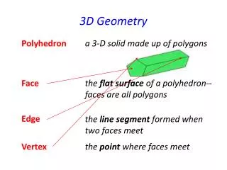
v4 t2 v1 (x1,y1, z1) (x2,y2, z2) v2 t1 v3 Some Mesh Preliminaries • Geometry • vertex1 = (x1, y1, z1) • vertex2 = (x2, y2, z2) • . . . • vertexv = (xv, yv, zv) • Incidence • Triangle1 = (vertex1, vertex2, vertex3) • Triangle2 = (vertex1, vertex2, vertex4) • . . . • We limit the discussion to simplemeshes—those that are topologically equivalent to a sphere. • An uncompressed representation uses 12v bytes for geometry and 12t bytes for incidence • Given that t ≈ 2v, 2/3 of the total representation costs goes to incidence
x x x x y y y y z z z z v1 v2 v3 v4 1 2 3 2 1 4 7 8 5 9 6 2 2 1 3 3 t0 2 t1 4 5 0 4 1 Corner Table: A Simple Mesh Data Structure • A naïve approach to storing a triangulated surface is as a list of independent triangles as described by 3 floating point coordinates. • Corner Table explicitly represents triangle/vertex incidence and triangle/triangle adjacency. V O G t0 c0 t0 c1 t0 c2 t1 c3 t1 c4 t1 c5
Corner Table: O-table • Corners associate a triangle with one of its vertices. • Cache the opposite corner ID in the O-table to accelerate mesh traversal from one triangle to its neighbors. • The O-table does not need to be transmitted because it can easily be recreated: For each corner a do For each corner b do if (a.n.v == b.p.v && a.p.v == a.n.v) O[a] = b O[b] = a Source: [2]
Geometry Compression: Quantization • Vertex coordinates are commonly represented as floats. • 3 x 32 bits per vertex geometry costs 96v bits • Range of values that can be represented may exceed actual range covered by vertices • Resolution of the representation may be more than adequate for the application. • Truncate the vertex to a fixed accuracy: • Compute a tight, axis aligned bounding box • Divide the box into cubic cells of size s • The vertices that fall inside a given cell are snapped to the center • Resulting error is bounded by the diagonal s s*2B
Geometry Compression: Quantization Gains • The number of bits required to encode each coordinate is less than B. • Empirically found that choosing B=12 ensures a sufficient geometric fidelity. • Simple quantization step thus reduces storage cost from 96v bits to 36v bits. original original 8 bits/coordinate 8 bits/coordinate
Geometry Compression: Prediction • Use previously decoded positions to predict the next positions • Store only the residue/offset between the predicted and actual positions to cut costs. (1008, 68, 718) – (1004, 71, 723) = (4, -3, -5) position prediction residue • The parallelogram construction for prediction is the most popular construction for single-rate compression. • Predict the next vertex’s position based on the previous triangle. d’ d d’ = a + b - c b a c
Connectivity Compression: Edgebreaker • Encodes connectivity using at most 2t bits: • Input: Triangulated mesh • Output: CLERS string • Initially define as the active boundary some arbitrary triangle • Boundary edges are initially those of the triangle • Uses a stack to temporarily store boundaries • The gate is defined to be one of the boundary edges • Both are directed counterclockwise around the triangle • Then visit every triangle in the mesh by including it in into an active boundary.
Edgebreaker Operations • 5 different operations are used to include a triangle into the active boundary Source: [3]
12 Final Operations of Edgebreaker Encoding Source: [3]
CRRRLSLECRE Source: [3]
Edgebreaker Encoding: Bottom Line • t = 2v – 4 2x more triangles than vertices • Half of all operations will be of type C • Thus encode C with one bit and the operations with 3 bits • C = 0 • L = 110 • E = 111 • R = 101 • S = 100 • Thus a simple CLERS string compression guarantees no more than 2t bits for storing the triangle mesh connectivity
Edgebreaker Decoding • Input: CLERS string Output: Triangulated mesh • Requires two traversals of CLERS string • Preprocessing: Compute offset values • Generation: Re-create triangles in the encoding order • Worst Case: O(n2) Source: [2]
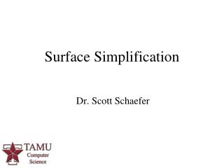
Surface Simplification • Level-of-details (LODs) refer to simplified models with a reduced number of triangles. • LODs can be sent initially to avoid transmission delays. • Refinements that upgrade fidelity can be sent later if needed. • Simplification techniques that reduce the triangle count while minimizing the introduced error are desired.
Surface Simplification: Vertex Clustering • Impose a uniformed, axis aligned grid on the mesh and cluster all the vertices that fall in the same cell. • Render all of the triangles in the original mesh with vertices replaced by a cluster representative • Choosing a representative vertex is non-trivial. • Preferable to use one of the actual vertices in the cluster. • Choosing the vertex closest to the average tends to shrink objects. • Empirically better to choose vertex furthest from the center of the bounding box.
Surface Simplification: Vertex Clustering • The maximum geometric error between the original and simplified shapes is bounded by the diagonal of each cell • Rarely offers the most accurate simplification for a given triangle count • Grid alignment may force 2 nearby vertices into different clusters and replace them with distant representatives 34,834 vertices 769 vertices Source: Image- Driven Mesh Optimization
Surface Simplification: Edge Collapsing • Collapsed triangles are easily removed from connectivity graph • Avoid topology-changing edge collapses • Select the edge whose collapse will have the smallest impact on the total error between the resulting mesh and the original surface • Error estimates must be updated after each collapse • Use priority queue to maintain list of candidates Source: [1]
Surface Simplification: Errors • Most simplification techniques are based on a view-independent error formulation. • E(A, B) = max. distance from all points/vertices p on A to B. • Yet this is not sufficient since that maximum error may occur inside a triangle and not at the vertices or edges.
Recap • Mesh geometry can be compressed in two steps: quantization and prediction. • The corner table data structure for meshes explicitly represents adjacency relations which can be exploited by algorithms that traverse a mesh. • Edgebreaker is a simple technique that can be used to compress mesh connectivity. • Simplification can further reduce file size, and the two main techniques are vertex clustering and edge collapsing. • All the techniques discussed are “barebones”—there are several optimizing variants.
References [1] J. Rossignac. Surface Simplification and 3D Geometry Compression. In Handbook of Discrete and Computational Geometry, 2nd edition, Chapman & Hall, 2004. [2] J. Rossignac, A. Safonova, and A. Szymczak. Edgebreaker on a Corner Table: A Simple Technique for Representing and Compressing Triangulated Surfaces. Presented at Shape Modeling International Conference, 2001. [3] M. Isenburg and J. Snoeyink. Spirale Reversi: Reverse decoding of the Edgebreaker encoding. Computational Geometry, 20: 39-52, 2001