Surface compression
This article compares different methods of lossy compression for surface data, focusing on the tradeoff between accuracy and processing time. Specifically, it explores the compression types, Fourier-related transform, quantization, entropy coding, and JPEG compression.

Surface compression
E N D
Presentation Transcript
Surface compression Comparison between methods of lossy compression Liad serruya
Motivation • Computer games and distributed virtual environments must often operate on systems where available resources are highly constrained. • At the high end realistic simulation and scientific visualization systems typically have object databases that far exceed the capacity of even the most powerful graphics workstations. • Tradeoff exists between the accuracy with which a surface is modeled and the amount of time required to process it.
Compression Types • Image compression • Surface simplification
Image compression • A Fourier-related transform such as DCT or wavelet transform. • Quantization techniques generally compress by transforming a range of values to a single quantum value. By reducing the number of discrete symbols in a given stream, the stream becomes more compressible. • Entropy encoders are used to compress data by replacing symbols represented by equal-length codes with symbols represented by codes proportional to the negative logarithm of the probability (Huffman coding, range encoding, and arithmetic coding). Fourier-related transform Quantization Entropy coding Image Compressed Image
Image compression Lost information • Chroma subsampling. This takes advantage of the fact that the eye perceives brightness more sharply than color, by dropping half or more of the chrominance information in the image. • Reducing the color space to the most common colors in the image. The selected colors are specified in the color palette in the header of the compressed image. Each pixel just references the index of a color in the color palette. This method can be combined with dithering to blur the color borders.
JPEG • In computing, JPEG (pronounced jay-peg) is the most commonly used standard method of lossy compression for photographic images. • It is not well suited for line drawings and other textual or iconic graphics because its compression method performs badly on these types of images.
JPEG – Compression schemes Color space transformation Downsampling Discrete Cosine Transform Image Quantization Entropy coding Decoding Compressed Image
JPEG – Color space transformation & Downsampling • First, the image is converted from RGB into a different color space called YCbCr. • The Y component represents the brightness of a pixel. • The Cb and Cr components together represent the chrominance. • This encoding system is useful because the human eye can see more detail in the Y component than in Cb and Cr. Using this knowledge, encoders can be designed to compress images more efficiently. • The above transformation enables the next step, which is to reduce the Cb and Cr components (called "downsampling" or "chroma subsampling").
JPEG – Discrete Cosine Transform • Each component of the image is "tiled" into sections 8×8 8-bit • Shifted by 128 • Taking the DCT and rounding to the nearest integer
JPEG – Quantization • The human eye not so good at distinguishing the exact strength of a high frequency brightness variation. This fact allows us to reduce the amount of information in the high frequency components. This is done by simply dividing each component in the frequency domain by a constant for that component, and then rounding to the nearest integer. This is the main lossy operation in the whole process.
JPEG – Quantization • A common quantization matrix • Using this quantization matrix with the DCT coefficient matrix from above For example, using −415 (the DC coefficient) and rounding to the nearest integer • As a result of this, the higher frequency components are rounded to zero, and the rest become small positive or negative numbers.
JPEG – Entropy coding • Special form of lossless data compression. It involves arranging the image components in a "zigzag" order employing Run Length Encoding (RLE) algorithm that groups similar frequencies together, inserting length coding zeros, and then using Huffman coding on what is left. • The zigzag sequence for the above quantized coefficients: −26, −3, 0, −3, −2, −6, 2, −4, 1, −4, 1, 1, 5, 1, 2, −1, 1, −1, 2, 0, 0, 0, 0, 0, −1, −1, 0, 0, 0, 0, 0, 0, 0, 0, … • JPEG has a special Huffman code word for ending the sequence prematurely when the remaining coefficients are zero. Using this special code word, EOB, the sequence becomes −26, −3, 0, −3, −2, −6, 2, −4, 1, −4, 1, 1, 5, 1, 2, −1, 1, −1, 2, 0, 0, 0, 0, 0, −1, −1, EOB
JPEG – Ratio and Artifacts • The resulting compression ratio can be varied according to need by being more or less aggressive in the divisors used in the quantization phase. Ten to one compression usually results in an image that can't be distinguished by eye from the original. 100 to one compression is usually possible, but will look distinctly artifact compared to the original. The appropriate level of compression depends on the use to which the image will be put.
JPEG – Decoding • Decoding to display the image consists of doing all the above in reverse. • Taking the DCT coefficient matrix and multiplying it by the quantization matrix from above. which closely resembles the original DCT coefficient matrix for the top-left portion. • Taking the inverse DCT results in an image with values and adding 128 to each entry
JPEG – Decoding • This is the uncompressed subimage. • Can be compared to the original subimage by taking the difference results in error values. • with an average absolute error of about 5 values per pixels. Compression Image Original Image Average absolute error
JPEG – Results • The above images show the use of lossy compression to reduce the file size of the image. • The first picture is 12,249 bytes. • The second picture has been compressed (JPEG quality 30) and is 85% smaller, at 1,869 bytes. Notice the loss of detail in the brim of the hat. • The third picture has been highly compressed (JPEG quality 5) and is 96% smaller, at 559 bytes. The compression artifacts are much more noticeable. • Ecent though the third image has high distortion, the face is still recognizable.
S3 Texture Compression (S3TC) • A group of related image compression algorithms originally developed by S3 Graphics, Ltd. • S3TC's fast random access to individual pixels made it uniquely suited for use in compressing textures in hardware accelerated 3D computer graphics. • S3TC is a lossy compression algorithm, resulting in image quality degradation, but for most purposes the resulting images are more than adequate.
S3TC – DXT1 • DXT1 is the smallest variation of S3TC, storing 16 input pixels in 64 bits of output, consisting of two 16-bit RGB 5:6:5 color values and a 4x4 two bit lookup table. • If the first color value c0 is numerically greater than the second color value c1, then two other colors are calculated, such that and . • Otherwise, if , then and c3 is transparent. • The lookup table is then consulted to determine the color value for each pixel, with a value of 0 corresponding to c0 and a value of 3 corresponding to c3. DXT1 does not support texture alpha data.
S3TC – Results 32 - bit S3TC – DXT1 Seems to have difficulty with gradients S3TC has much weaker grid
Efficiency and quality of different lossy compression techniques The performances of lossy picture coding algorithms are usually evaluated on the basis of two parameters: • The compression factor (or analogously the bit rate) – objective parameter. • d • D • The distortion produced on the reconstruction – strongly depends on the usage of the coded image.
Motivation – Surface simplification • Tradeoff exists between the accuracy with which a surface is modeled and the amount of time required to process it. • A model which captures very fine surface detail helps ensure that applications which later process the model have sufficient and accurate data. • However, many applications will require far less detail than is present in the full dataset. • Surface simplification is a valuable tool for tailoring large datasets to the needs of individual applications and for producing more economical surface models.
QSlim • The simplification algorithm is a decimation algorithm. It begins with the original surface and iteratively removes vertices and faces from the model. Each iteration involves the application of a single atomic operation: • A vertex pair contraction, denoted by (vi; vj) v, modifies the surface in three steps: • Move the vertices vi and vj to the position v; • Replace all occurrences of vj with vi; • Remove vj and all faces which become degenerate – that no longer have three distinct vertices.
QSlim Edge (vi; vj) is contracted. The darker triangles become degenerate and are removed. • Non-edge pair (vi; vj) is contracted, joining previously unconnected areas. No triangles are removed.
QSlim • The algorithm, like most related methods, is a simple greedy procedure. It produces large-scale simplification by applying a sequence of vertex pair contractions. This sequence is selected in a purely greedy fashion. once a contraction is selected, it is never reconsidered. The outline of the algorithm is as follows: • Select a set of candidate vertex pairs. • Assign a cost of contraction to each candidate. • Place all candidates in a heap keyed on cost with the minimum cost pair at the top. • Repeat until the desired approximation is reached: • Remove the pair (vi; vj) of least cost from the heap. • Contract this pair. • Update costs of all candidate pairs involving vi.
QSlim Simplification of a simple planar object. Vertex correspondences
Comparison • Image matrix => Triangulation => QSlim => Compressed Triangulation => Compressed Image matrix QSlim Triangulation Triangulation
Future work • QSlim can be compressed further by standard lossless compression techniques, such as ZIP • Create Comparison application between Image compression and Surface simplification compression
Good lossy compression algorithms are able to throw away "less important" information and still retain the "essential" information.