Compression Techniques for Data Transfer Optimization
Learn about compression techniques to reduce data size for efficient transfer, including lossless vs. lossy methods, entropic coding, and source encoding. Explore examples like run-length and statistical encoding, as well as techniques such as differential and transform encoding. Discover how JPEG compression optimizes data for multimedia applications.

Compression Techniques for Data Transfer Optimization
E N D
Presentation Transcript
Compression There is need for compression: bandwidth constraints of multimedia applications exceed the capability of communication channels Ex. QCIF bit rate: 40.5 Mbps (IEEE 802.11b: 11 Mbps!!!) There is need for reducing the amount of data to be transferred to limit cost of communication infrastructures compression techniques
Compression 101 • For compression to be implemented we need a coder and a decoder. They apply some transformations on the data to be transmitted at one side of the transmission medium (coder) and reconstruct the information at the other end of the transmission medium (decoder). • The transformation can be: “lossless” (reversible) and “lossy” We will examine two types of coding: • Entropic coding • Lossless, independent from the type of information • Says how to represent the information to be transmitted • Source coding • Exploits characteristics of information content
Lossless VS Lossy “Lossless” compression is reversible. A typical application could be compression of a text file to be transferred over the network. “Lossy” compression cause some information to be lost, so that the decoder can only perform an approximate reconstruction of the original information. It usually achieves an higher compression ratio than lossless coding. Moreover, to obtain larger compression ratio a larger error have to be tolerate. To reduce the impact of this error, these techniques try to perform a smart approximation, that is the information that is discarded is the less important for the user. This principle is called perceptual coding, because these techniques try to reduce the distortion perceived by the user (for example when compressing an image or an audio stream)
Entropic Coding Entropic coding is lossless and INDEPENDENT from information type, it is only related on how information is represented, no matter what the content is. • There are two common examples of entropic coding: • Run-length encoding • Statistical encoding
Run-Length Encoding • Applicability: The information includes very long sub-strings of the same character • Idea: Transmit “codewords” that can be understood by the decoder and indicate: • the character that is repeated • the number of characters in the sub-string • Requisite: The decoder knows the codeword set • Ex. 000000011111111110000011……….. • 0,7,1,10,0,5,1,2,… B) 7,10,5,2,…. • (binary converted using a constant number of bit for each codeword) • In the second case, the information about the type of bit is implicit because they are alternated.
Statistical Encoding • Applicability: Transmission of symbols with a constant number of bits (Ex. ASCII symbols of 7 bit) • Idea: The binary coding is reassigned so that less bit are used for frequent symbols (variable length codewords) • Requisite: • The decoder knows the codeword set • “Short codewords” are not prefix of “long codewords” (PREFIX propriety: ex. Huffman coding follows this rule)
Source Encoding A particular propriety of the source is exploited to give an alternative representation that is more compressed than the original one or more suitable to compression • Two common used techniques: • Differential encoding • Transform encoding
Differential Encoding Instead of representing the absolute value of a quantity (with large range) the difference is represented between a value and the previous one (thus limiting the range) Example: digitalize an analog value that requires 12 bits: if the difference requires only 3 bits up to 75% of bandwidth can be saved This kind of compression can be or lossy depending on the number of used for the difference
Transform Encoding In this technique it is used a change of domain that does not imply information losses to enhance compression Example: The spatial frequency is the rate of variation observed in the scanning of matrix of pixels along one direction. Note that on the spatial frequency domain components with the same pixel intensity are mapped to different frequency depending on their spatial variation
Transform Encoding • After the domain switch, we can more easily perform a lossy compression that treats better the information which is more relevant (e.g. in video coding): • The eye is less sensitive to high spatial frequencies • If the amplitude of a high frequency component falls below a certain threshold, the eye does not detect it Quantization can be less accurate at higher frequencies (= less bit)
JPEG Joint Photographic Experts Group • Here we see an example of a complex compression scheme that exploits several types of coding techniques. • We have different versions • Lossy sequential mode (or baseline mode) • Progressive encoding • Baseline JPEG is based on the following steps: • Image preparation • DCT • Quantization • Entropic coding • Frame composition
Image Preparation Different input formats Representation in reduced form 8 BIT/PIXEL Y: 0..255 U,Cb,Cr: -128 ..+127
Block Preparation Performing the DCT on all the matrix is too expensive: block subdivision 2D-DCT on 8x8 blocks
Forward DCT • All of 64 pixels of the input matrix contribute to DCT. • DC coefficient F[0,0] represent the average of pixel values, while AC coefficients represent the spatial frequency along rows or columns • For j=0, AC horizontal coefficients with increasing frequency • For i=0, AC vertical coefficients with increasing frequency • In the remaining locations, there is contribution of components both for vertical and horizontal frequency
Some Comments • Block size: Let us consider 640x480 pixels images (4:2:0 at 525 lines). With block size of 8x8 pixels we have 4800 blocks that on a 400mm screen occupy 5x5mm. • Value of coefficients: inside an image we typically have monochromatic regions and regions with color transitions • Monochromatic regions: • DCT blocks with similar DC coeff. • a few AC coeff. that are NOT zero • Regions with color transitions • various DC coeff. • a large number of AC coeff. that are NOT zero Entropic quantization and coding
JPEG Compression • In JPEG, the compression happens in ENTROPIC QUANTIZZAZATION and CODING phases. • It exploits characteristics of the human eye: • The eye is more sensitive to DC component and AC with low frequency • In practice, a threshold is set. If a coeff is under the threshold it is deleted. Instead of a simple threshold comparison, a division is performed to reduce bandwidth of transmission. The divisor represents the threshold. The drawback is the loss of accuracy.
Very high value At HF several Coeff are null Quantization: DIVISION by a threshold and round-up
Quantization Tables The threshold at which the eye detect a spatial frequency varies depending on the frequencye • 2 quantization tables specified by JPEG standard • It is possible to customize the tables • In the threshold choice there is a trade-off between compression and information loss
Entropic Coding Entropy coder Differential encoding To Frame Builder From quantizer Vectoring Huffman encoding Run-length encoding Tables
Differential encoding Run length coding Vectoring Monodimensional vectors are formed Entropic coding 2D matrix from quantization Row-by-row scanning is not suitable to compression, then a zig-zag scanning is performed 63 2 1 0 AC DC There are long sequences of zeros
Differential Encoding For DC coefficients: • Quantization with higher precision • It does not vary too much from block to block, being the block small • Differential encoding is more applied 12,1,-2,0,-1,… Ex. 12,13,11,11,10,…. • Coding in the form (SSS,value) • SSS: number of bits needed to code the value value: the amount of the difference • value is binary coded, SSS is coded with Huffman coding
Variable Length Coding Binary if positive Complement if negative Codifica del DC coeff. Difference SSS value 0 0 -1,1 1 1=1, -1=0 -3,-2,2,3 2 2=10, -2=01 3=11, -3=00 -7,..,-4,4..,7 3 4=100, -4=011 5=101, -5=010 ………………….. -15,..,-8,8,..,15 4 8=1000, -8=0111 ……………………
Huffman Coding for DC Coefficients Huffman table for DC coefficients SSS
Run Length Coding • For AC coefficients: • coded as a couple (skip,value) • Skip: number of zeros in the run • Value: value of the next NOT NULL coefficient Example: Zig zag ordered DC 0……0 0 0 2 2 2 2 3 3 3 7 6 12 (0,6) (0,7) (0,3) (0,3) (0,3) (0,2) (0,2)(0,2) (0,2) (0,0) • block end • Remaining coeff are null • value is coded as (SSS,value) • skip is coded with Huffman (together with SSS)
Coding of skip and SSS • Skip and SSS are treated as a single symbol coded with Huffman Ex. 3/2 corresponds to 111110111 • How the decoder distinguishes between Skip and SSS? Each combination (Skip, SSS) is coded separately with Huffman • Ex. 3/2 111110111 • 3/3 11111110111 • ………………….
Progressive Encoding • It allows to transmit a rough version of the image with low rate and then progressively improves the quality with successive transmissions (used in web-browsing) • Two methods: • Spectral selection • Sets of DCT coeff are sent starting from low frequencies and progressively upgrading to higher frequencies • Successive approximation • The first n1bit more significant are sent, then n2 bit, etc… • All the frequencies at the same time are transmitted
Mixed Approach • A combination of the two approaches can be used • All of the bits for DC coefficients • Reduction of precision for AC coefficients • Rate = 0.24bit/pixel • It achieved better quality w.r.t. to pure spectral selection at 0.36bit/pixel. DC and first 5 AC coefficients are transmitted at full precision.