Download
1 / 30
340 likes | 1.46k Vues
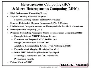
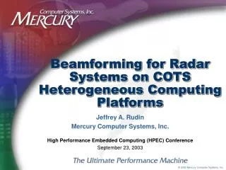
Beamforming for Radar Systems on COTS Heterogeneous Computing Platforms. Jeffrey A. Rudin Mercury Computer Systems, Inc. High Performance Embedded Computing (HPEC) Conference September 23, 2003. Outline. Beamforming Radar System Architecture Processing Resources Strawman System Analysis

E N D
Beamforming for Radar Systems on COTS Heterogeneous Computing Platforms Jeffrey A. Rudin Mercury Computer Systems, Inc. High Performance Embedded Computing (HPEC) Conference September 23, 2003
Outline • Beamforming Radar System Architecture • Processing Resources • Strawman System Analysis • Front-End Processing • Back-End Processing • Beamformer Architectures • Summary
Sub-Array Beamformer Pulse Compression Pulse Compression Pulse Compression Pulse Compression Pulse Compression Adaptive Beamformer Adaptive Beamformer Adaptive Beamformer Adaptive Beamformer Adaptive Beamformer RF Combiner RF Combiner RF Combiner RF Combiner RF Combiner ADC ADC ADC ADC ADC Front-End Front-End Front-End Front-End Front-End m-P ANALOG FPGA Digital Memory Radar System Architecture • Beamforming requires massive dataflow and computation • ADC precision and data rate are chosen to provide high dynamic range and and wide signal bandwidth • High number of input channels required in modern phased array radars to produce multiple beams and nulls
Processing Resources • Microprocessors • Fixed processing, I/O, and memory architecture • Task context switch requires microseconds • Native floating-point available • Low interaction between code modules • FPGAs • Customizable processing, I/O, and memory architecture • Task context switch requires reconfiguration -- milliseconds • Floating-point must be built or bought • Considerable interaction between IP cores • Signal propagation issues • Currently harder to program than microprocessors
ARITHMETIC UNIT VECTOR ALU FLOATING-POINT ALU INTEGER ALU INSTRUCTION UNIT MEMORY CONTROL UNIT DISPATCH UNIT LOAD/STORE UNIT BRANCH PROCESSING DATA MMU INSTRUCTION MMU DATA CACHE INSTRUCTION CACHE COMPLETION UNIT MEMORY SUBSYSTEM L2 CONTROLLER BUS INTERFACE UNIT PowerPC Microprocessor • 400 - 1000 MHz clock speeds • 133 MHz system bus (MPC74xx) -- 851 MB/s • 64-bit integer and floating-point units • 128-bit AltiVec vector processing unit • Pipelined instruction unit • 32 kB instruction and data caches • Up to 2 MB L2 cache
I/O BLOCKS DEDICATED MULTIPLIERS REGISTERS LUT’S CARRY LOGIC MULTIPLEXERS DISTRIBUTED RAM SHIFT REGISTERS PowerPC 405 CORE CONFIGURABLE LOGIC CLOCK MANAGERS DUAL-PORT BLOCK RAM FULL DUPLEX TRANCEIVERS Virtex-II Pro FPGA • Clock speeds lower than processors: 100 - 200 MHz clocks • Up to 20 full-duplex multi-gigabit transceivers. • Many DSP supporting features Each block RAM contains two banks with independent sets of address and data lines Gigabit transceivers provide over 240 MBps each direction -- over 4800 MBps throughput!
184 188 160 ANALOG/DIGITAL CONVERTER DATA RATES INPUT CHANNELS PER FPGA USING GIGABIT Tx/Rx 158 130 140 50 50 200 40 114 43 120 40 31 35 150 26 37 27 98 30 30 100 Maximum Input Channels Data Rate (MByte/sec) 20 50 10 12-bit 16-bit 0 0 14-bit 14-bit 125 MHz 12-bit 125 105 MHz 16-bit 105 80 MHz 65 MHz 80 65 MHz MHz MHz MHz Strawman System Requirements • Lots of channels -- 80+ input channels • ADC with “good” bandwidth and dynamic range • 100 MSps -- 1.56 - 25 MHz bandwidth using fs/4 sampling • 14-bit precision -- over 80 dB dynamic range • Reasonable implementation risk -- 100 MHz clock ADC precision and rate and number of channels drive downstream requirements
Front-End Processing • Digital Down Converter • fs/4 IF & BW • 4x decimation • 31-tap complex FIR, real symmetric coefficients • Usually no bit growth • Lowpass Decimation Filter • 1x (bypass), 2x, 4x, 8x, and 16x decimation rates • 0, 16, 32, 64, 128 taps • Real coefficients • 0 to 2 bits of bit growth • Equalizer • 16-tap, complex coefficients -- cannot generally exploit symmetry • Usually no bit growth Eliminates the need for numerically controlled oscillators (NCO)
Q h0 h4 h8 h12 h14 h10 h6 h2 + POLYPHASE fs/4 DDC h1 h5 h9 h13 h13 h9 h5 h1 h2 h6 h10 h14 h12 h8 h4 h0 I + h3 h7 h11 h15 h11 h7 h3 Digital Down Converter • Reduce complexity -- exploit fs/4 center frequency and bandwidth • Complex mixing reduces to polyphase commutation • Cosine and sine select even and odd samples respectively • cos(jnp/4) = 1, 0, -1, 0, 1,…; sin(jnp/4) = 0, j, 0, -j, 0,… • Exploit polyphase structure for decimation Odd number of taps creates symmetries in the FIR coefficients
+ + + + S + + + + S Digital Down Converter • Reduce complexity -- exploit filter symmetries Exploit symmetric filter structures for in-phase signal Exploit symmetry pair filters for quadrature signal Each tap calculation involves one coefficient and two samples
SRL-16 SRL-16 x[n] + + BRAM h[n] x1[n] SRL-16 SRL-16 x2[n] + + BRAM h[n] Digital Down Converter • Reduce complexity -- exploit 4x decimation • Use MAC-Engine to do 4 multiplies per input sample • Use fclk = 4 x fs to time share multipliers • Configure logic slices as shift registers (SRL’s) to save BRAM • Need to store 3 sets of numbers -- need 2 BRAM’s • Save BRAM by using logic slices to store both sets of samples Symmetry Filter Pair Symmetric Filter
MAC-Engine MAC-Engine x[n] BRAM BRAM + + + h[n] h[n] Low Pass Filter • Reduce complexity -- use MAC-Engine FIR implementation • Run multipliers at 4x sample rate -- time share multipliers • Exploit constant length-decimation product • Single structure handles multiple filter implementations • Single clock frequency • Use dual-bank feature of BRAM • First bank stores samples • Second bank stores FIR coefficients
(hr+ hi) yi + + xr + yr + xi + (hr- hi) yi Trade logic slices for block RAM Trade logic slices for multipliers + + hr + hr xr + hi xi + yr + + Equalizer • Reduce complexity --reduce number of multipliers and BRAM’s • Exploit fclk/fs -- use MAC-Engine • Implement complex multiply using only 3 MAC-Engines • Use common product term in complex multiply
Processing I/O Memory Ctrl. Margin Channels 1-20 100 MByte/s 9x 2.5 Gb FO Channels 1-20 200 MByte/s 20x 2.5 Gb FO From ADC’s DDC DDC DDC DDC LPF LPF LPF LPF EQU EQU EQU EQU Additional copy of each channel for distribution Block Ram Logic Slices Multipliers Front-End Realization • FPGA features can be exploited to maximize utilization • Up to 20 100-MSps channels per FPGA • DDC with 31-Tap FIR using only 3 multipliers/channel • LPF 16-128 Tap decimating FIR using only 4 multipliers/channel • EQU 16-Tap complex FIR using only 12 multipliers/channel Digital Receiver Module for 20x 100 MSps Channels on Virtex-II Pro 100 HIGH FPGA UTILIZATION FPGA Utilization for 20x 100 MSps Channels
Back-End Processing • FPGAs can be used to address data flow requirements that persist in the system until application of adaptive beamforming weights • Digital Pulse Compression • Fast convolution with FFT IP cores • Doppler Processing • FPGA FFT IP cores available • Adaptive Beamforming Weight Application • Similar advantages to those in sub-array beamformer • FPGAs can augment weight computation • QR Decomposition • New FPGA solutions may replace microprocessors • Cholesky Decomposition • Possibly form covariance matrix in adjunct FPGA
Memory Memory Partial Product 1 SUM I/O FFT MUL IFFT Partial Product 2 FFT MUL IFFT Multipliers Block Ram Logic Slices Processing I/O Memory Ctrl. Margin Digital Pulse Compression • FFT IP cores can be used to implement pulse compression • 8192-tap FFT @ 25 MSps/channel • 6 sub-array channels / FPGA • 3-stage pipelined convolver -- 2 convolvers / FPGA • Enough resources to sum partial products from beamformer Doppler processing can be implemented using similar FFT cores GOOD FPGA UTILIZATION DIGITAL PULSE COMPRESSION FPGA UTILIZATION FFT cores tend to be BRAM hungry.
Beamformer Architectures • Unconstrained Linear Architecture • All input channels contribute to each output • Constrained Linear Architecture • A subset of input channels contributes to any output • Mesh Architecture • All input channels contribute to each output
I/O and Multiplier Constraints for Virtex-II Pro 100 1000 100 Number of Output Channels USEABLE CONFIGURATIONS 10 Assumes: 3-MAC / CMAC 25 MSps channels 100 MHz clock 1 1 10 100 Number of Input Channels Beamformer Module Constraints • Basic limits are imposed by I/O and number of multipliers • Inputs over 18-bits can increase the number of multipliers • Keep watch on bit growth in front-end processing
12 24 100 14 20 40 90 8 22 36 80 10 32 38 70 18 28 34 60 16 Multiplexing Efficiency 30 50 26 40 30 20 10 0 0 10 20 30 40 Number of Channels per Beam Beamformer Module Constraints • Multiplexing must be designed to maximize communication • Beam Partitioned output multiplexing may reduce efficiency • Alternate multiplexing methods may be necessary Data can also be partitioned by link: each link carried an integral number of channels
Beamformer Digital Rx Input Sets Beams CPI CPI PROC PROC PROC PROC PROC PROC NPasses Memory Unconstrained Linear Architecture • Full MxN unconstrained complex matrix multiply • Outputs only from a single module • Processing throughput limited by beamformer module I/O • Communication latency across beamformer is an issue • Additional beams can be produced by multiple passes on data • Decreases overall radar duty cycle • Memory should be located in digital beamformer to save I/O bandwidth • Increased beamformer processing speed may be required
1000 COMPUTATIONAL LIMIT 100 Number of Output Channels COMMUNICATION LIMIT 4 input module 10 USEABLE CONFIGURATIONS 20 input module 1 1 10 100 Number of Input Channels Unconstrained Linear Architecture • Unconstrained linear beamformer module is I/O bound • Total number of input links plus output links is constant • Choice of input to output balance affects utilization Note:adding additional non-MGT connections could potentially increase throughput
DPC DPC 96 36 36 DPC 8.4 GBps 5.9 GBps DPC DPC Beamform DPC Beamform Multipliers Block Ram Logic Slices Processing Digital Rx Beamform 20 4 I/O Memory Ctrl. Margin Beamform Beamform BEAMFORMER MODULE UTILIZATION 4 Input Module Realization • I/O and compute bounds are not close -- low utilization • 36 x 96 unconstrained matrix multiply • 35 modules required for FPGA digital processor • Front-end – 5 modules • Small-array beamformer – 24 modules • Digital pulse compression – - 6 modules LOW FPGA UTILIZATION
Multipliers Block Ram Logic Slices Digital Rx 20 Digital Rx 20 BEAMFORMER MODULE UTILIZATION Digital Rx 20 Digital Rx 20 DPC DPC Digital Rx 20 Beamform 20 DPC 100 100 40 40 8.8 GBps 20 DPC Beamform 20 20 DPC Beamform 20 DPC 20 Beamform 20 DPC 20 Beamform 20 20 Processing I/O Memory Ctrl. Margin 20 Input Module Realization • I/O and compute bounds are close -- good utilization • 40 x 100 unconstrained matrix multiply • 22 modules required for FPGA digital processor • Front-end – 5 modules • Small-array beamformer – 10 modules • Digital pulse compression – 7 modules 6.5 GBps GOOD FPGA UTILIZATION
Beamformer Digital Rx 1000 COMPUTATION LIMIT COMMUNICATION LIMIT 100 Number of Output Channels 10 USEABLE CONFIGURATIONS 1 Memory 1 10 100 Number of Input Channels Constrained Linear Architecture • Use each beamformer module to produce outputs • MxN constrained complex matrix multiply • Use only a subset of inputs for each output • I/O and computation bounds the as in the unconstrained case • Inputs and outputs must be balanced to maximize utilization EXPLICIT ZEROS IN BEAMFORMING MATRIX
Beamform Beamform Beamform Beamform Beamform Digital Rx Digital Rx Digital Rx Digital Rx Digital Rx 20 20 20 20 20 20 20 20 20 20 20 20 20 20 20 20 Multipliers Block Ram Logic Slices 10 10 10 10 BEAMFORMER MODULE UTILIZATION DPC DPC 10 DPC DPC 50 50 100 8.8 GBps 8.1 GBps DPC DPC DPC DPC DPC Processing I/O Memory Ctrl. Margin 20 Input Module Implementation • Adding matrix constraints increases the number of outputs • 50 x 100 constrained matrix multiply • 19 modules required for FPGA digital processor • Front-end - 5 modules • Small-array beamformer – 5 modules • Digital pulse compression - 9 modules GOOD FPGA UTILIZATION
5 links 10 channels 5 links 10 channels 5 links 12 channels 5 links 12 channels 1000 COMPUTATION LIMIT 5 links 12 channels 5 links 12 channels 100 Number of Output Channels COMMUNICATION LIMITS 10 USEABLE CONFIGURATIONS 5 links 10 channels 5 links 10 channels 1 1 10 100 Number of Input Channels Mesh Architecture • Mesh architecture offers utilization enhancement • I/O and computation bounds touch • Full unconstrained matrix multiply • Partially formed beams sent forward for summing in DPC NO EXPLICIT ZEROS IN BEAMFORMING MATRIX 40 x 48 CMAC using 4 modules Note: Computation limit normalized for architecture
Multipliers Block Ram Logic Slices BEAMFORMER MODULE UTILIZATION DPC DPC Digital Rx DPC 96 96 40 40 8.4 GBps 6.5 GBps DPC Digital Rx DPC Digital Rx DPC Digital Rx DPC Digital Rx Processing I/O Memory Ctrl. Beamform Margin Beamform Beamform Beamform Mesh Implementation • I/O and compute bounds touch -- high utilization • 40 x 96 unconstrained matrix multiply • 20 modules required for FPGA digital processor • Front-end – 5 modules • Small-array beamformer – 8 modules • Digital pulse compression – 7 modules HIGH FPGA UTILIZATION
Architecture Comparison • Mesh architecture gives highest multiplier utilization
Channels 1-160 Channels 1-96 Large Systems • Large systems can be created through layering beamformers • 8 beam system, 20 channels per beam -- 160 channels • 160 x 96 unconstrained matrix multiply • 65 modules required for FPGA digital processor • Front-end - 5 modules • Small-array beamformer – 32 modules • Digital pulse compression - 28 modules
Summary • FPGAs can provide efficient I/O and computational power to address high input bandwidths of modern radar systems. • Front-end processing • Sub-array beamformer • Digital pulse compression • Adaptive beamforming • System topologies that provide efficient utilization of computational and I/O resources change dramatically as system requirements scale. • Watch I/O and computation bounds • Small changes in system requirements can dramatically increase complexity of FPGA implementations when computational bounds of embedded resources is exceeded. • Watch for symmetries in filters • Watch bit growth before 18-bit multipliers • FPGAs should be used until application of adaptive beamforming weights due to high bandwidth dataflow.