Load Balancing Parallel Applications on Heterogeneous Platforms
280 likes | 523 Vues
Load Balancing Parallel Applications on Heterogeneous Platforms. Heterogeneous Platforms. So far we ’ ve only talked about platforms in which all processors/nodes are identical representative of most supercomputers Clusters often “ end up ” heterogeneous Built as homogeneous

Load Balancing Parallel Applications on Heterogeneous Platforms
E N D
Presentation Transcript
Load Balancing Parallel Applications on Heterogeneous Platforms
Heterogeneous Platforms • So far we’ve only talked about platforms in which all processors/nodes are identical • representative of most supercomputers • Clusters often “end up” heterogeneous • Built as homogeneous • New nodes are added and have faster CPUs • A cluster that stays up 3 years will likely have several generations of processors in it • Network of workstations are heterogeneous • couple together all machines in your lab to run a parallel applications (became popular with PVM) • “Grids” • couple together different clusters, supercomputers, and workstations • It is important to develop parallel applications that can leverage heterogeneous platforms
Heterogeneous Load Balancing • There is an impressively large literature on load-balancing for heterogeneous platforms • In this lecture we’re looking only at “static” load balancing • before execution we know how much load is given to each processor • e.g., as opposed to some dynamic algorithm that assigns work to processors when they’re “ready” • We will look at: • 2 simple load-balancing algorithms • application to our 1-D distributed image processing application • application to the 1-D distributed LU factorization • discussion of load-balancing for 2-D data distributions (which turns out to be a very difficult problem) • We assume homogeneous network and heterogeneous compute nodes
Static task allocation • Let’s consider p processors • Let t1,..., tp be the “cycle times” of the processors • i.e., time to process one elemental unit of computation (work units) for the application (Tcomp) • Let B be the number of (identical) work units • Let c1,..., cp be the number of work units processed by each processor c1 + ... + cn = B • Perfect load balancing happens if cix ti is constant or computing speed
Static task allocation • if B is a multiple of then we can have perfect load balancing • But in general, the formula for ci does not give an integer solution • There is a simple algorithm that give the optimal (integer) allocation of work units to processors in O(p2)
Simple Algorithm // initialize with fractional values // rounded down For i = 1 to p // iteratively increase the ci values while (c1 + ... + cp < B) find k in {1,...,p} such that tk(ck + 1) = min {ti(ci + 1)} ck = ck + 1
Simple Algorithm p1 p2 p3 • 3 processors • 10 work units p1 p2 p3 c1 = 5 c2 = 3 c3 = 2 8 5 3
An incremental algorithm • Note that the previous algorithm can be modified slightly to record the optimal allocation for B=1, B=2, etc... • One can write the result as a list of processors • B=1: P1 • B=2: P1, P2 • B=3: P1, P2, P1 • B=4: P1, P2, P1, P3 • B=5: P1, P2, P1, P3, P1 • B=6: P1, P2, P1, P3, P1, P2 • B=7: P1, P2, P1, P3, P1, P2, P1 • etc. • We will see how this comes in handy for some load-balancing problems (e.g., LU factorization)
Image processing algorithm 0 1 2 3 4 5 6 7 8 9 10 11 12 13 11 2 5 6 7 8 9 10 13 3 4 11 12 14 15 3 4 5 6 7 8 9 10 15 16 11 12 13 14 5 6 7 8 9 10 11 12 13 14 15 17 18 n = 44, p= 4, r = 3, k = 4 13 14 15 16 16 First block Second block k = width of the parallelograms r = height of the parallelograms (number of rows per processors)
On a heterogeneous platform • Compute a different r value for each processor using the simple load-balancing algorithm • pick B • compute the static allocation • allocate rows in that pattern, in a cyclic fashion • Example • B = 10 • t1 = 3, t2 = 5, t3 = 8 • allocation: c1 = 5, c2 = 3, c3 = 2 5 rows . . . 3 rows 2 rows
LU Decomposition requires load-balancing max aji needed to compute the scaling factor to find the max aji Independent computation of the scaling factor Compute Reduction Broadcast Every update needs the scaling factor and the element from the pivot row Independent computations Broadcasts Compute
Load-balancing • One possibility is to directly use the static allocation for all columns of the matrix Processor 2 is idle Processor 1 is underutilized
Load-balancing • one possibility is the rebalance at each step (or each X steps) Redistribution is expensive in terms of communications
Load-balancing • Use the distribution obtained with the incremental algorithm, reversed • B=10: P1, P2, P1, P3, P1, P2, P1, P1, P2, P3 . . . optimal load-balancing for 10 columns optimal load-balancing for 7 columns optimal load-balancing for 4 columns
Load-balancing • Of course, this should be done for blocks of columns, and not individual columns • Also, should be done in a “motif” that spans some number of columns (B=10 in our example) and is repeated cyclically throughout the matrix • provided that B is large enough, we get a good approximation of the optimal load-balance
2-D Data Distributions • What we’ve seen so far works well for 1-D data distributions • use the simple algorithm • use the allocation pattern over block in a cyclic fashion • We have seen that a 2-D distribution is what’s most appropriate, for instance for matrix multiplication • We use matrix multiplication as our driving example
2-D Matrix Multiplication • C = A x B • Let us assume that we have a pxp processor grid, and that p=q=n • all 3 matrices are distributed identically Processor Grid
2-D Matrix Multiplication • We have seen 3 algorithms to do a matrix multiplication (Cannon, Fox, Snyder) • We will see here another algorithm • called the “outer product algorithm” • used in practice in the ScaLAPACK library because • does not require initial redistribution of the data • is easily adapted to rectangular processor grids, rectangular matrices, and rectangular blocks • as usual, one should use a blocked-cyclic distribution, but we will describe the algorithm in its non-blocking, non-cyclic version
Outer-product Algorithm • Proceeds in k=1,...,n steps • Horizontal broadcasts: Pi,k, for all i=1,...,p, broadcasts aik to processors in its processor row • Vertical broadcasts: Pk,j, for all j=1,...,q, broadcasts akj to processors in its processor column • Independent computations: processor Pi,j can update cij = cij + aikx akj
Load-balancing • Let ti,j be the cycle time of processor Pi,j • We assign to processor Pi,j a rectangle of size ri x cj c1 c2 c3 r1 r2 r3
Load-balancing • First, let us note that it is not always possible to achieve perfect load-balacing • There are some theorems that show that it’s only possible if the processor grid matrix, with processor cycle times, tij, put in their spot is of rank 1 • Each processor computes for rix cjx tij time • Therefore, the total execution time is T = maxi,j {rix cjx tij}
Load-balancing as optimization • Load-balancing can be expressed as a constrained minimization problem • minimize maxi,j {rix cjx tij} • with the constraints
Load-balancing as optimization • The load-balancing problem is in fact much more complex • One can place processors in any place of the processor grid • One must look for the optimal given all possible arrangements of processors in the grid (and thus solve an exponential number of the the optimization problem defined on the previous slide) • The load-balancing problem is NP-hard • Complex proof • A few (non-guaranteed) heuristics have been developed • they are quite complex
“Free” 2-D distribution • So far we’ve looked at things that looked like this • But how about?
Free 2-D distribution • Each rectangle must have a surface that’s proportional to the processor speed • One can “play” with the width and the height of the rectangles to try to minimize communication costs • A communication involves sending/receiving rectangles’ half-perimeters • One must minimize the sum of the half-perimeters if communications happen sequentially • One must minimize the maximum of the half-perimeters if communications happen in parallel
Problem Formulation • Let us consider p numbers s1, ..., sp such that s1+...+sp = 1 • we just normalize the sum of the processors’ cycle times so that they all sum to 1 • Find a partition of the unit square in p rectangles with area si, and with shape hixvi such that h1+v1 + h2+v2 + ... + hp+vp is minimized. • This problem is NP-hard
Guaranteed Heuristic • There is a guaranteed heuristic (that is within some fixed factor of the optimal) • non-trivial • It only works with processor columns