Multiple regression, ANCOVA, General Linear Models

1. Multiple regression, ANCOVA, General Linear Models

2. Multiple regression

3. I have more predictors than one • In manipulative experiment – amount of water and dose of nutrients as independent variables for biomass of plant raised • In observation study – species richness is explained by latitude, altitude and annual rainfall.

4. In ideal case, predictors shouldn’t be correlated with each other • This can be ensured in an experiment • But hardly in observational study (e.g., it would be difficult to find a locations ina way that latitude and precipitation would be independent)

5. Model The same assumptions as in simple linear regression – i.e. random variability is additive and independent of the expected value (i.e. homogeneity of variances), relation is linear. More over - effects of individual independent variables are additive.

6. For two predictors is representation a plain in three-dimensional space [ozone] Temperature Wind velocity

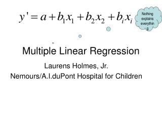
7. Numbers of procedures are analogue to simple regression • coefficients α and βi(for each of predictors) mean value for the population, [which is unknown], we estimate using a sample coefficients a and bi. • βi (for population), or bi. for sample - slope (dependent on units used) • Criterion of least squares of residual sum of squares. • Tests - either ANOVA of the whole model, or (using t-tests) tests of individual regression coefficients

8. In contrast to single regression, meaning of tests differs • ANOVA of the whole model: H0: Response is independent of all the predictors, i.e. βi=0 for all i • Separate null hypothesis for individual predictors βi=0 – relating to individual variables.

9. Range of predictor values can differ considerably. and slope values are dependent on units used. Water Nutrients P.High

10. ANOVA of whole model Analysis of sum of squares SSTOT = SSRegress. + SSResidual DFTOT = n-1 ; DFRegress=number of variables, DFResid=n-1-number of variables Classically MS=SS/DF = is estimation of population variance, if H0 is true – this all leads to classic F-distribution.

11. R2 - coefficient of determination Percentage of variability explained by model R2adj. = adjusted – different corrections; having many independent variables and relatively few observations, then R2 is higher in our sample than in the population. Number of observations should be considerably higher than no. of predictors. When number of observations = number of predictors + 1, then the model perfectly fits all points, (but predictive ability of the model is null).

12. Partial regression coefficients How much explains given variable in addition to all other variables in the model (“in addition” is especially important to say, if predictors are correlated)

13. Tests of partial regression coefficients Beta in Statistica program – it is something different than “our” β - (on principle, it cannot be computed from finite sample). It is standardized partial regression coefficient (computed after Z transformation of all the variables (both predictors and response) Regression plain goes through the origin thereafter

14. Tests of partial regress coefficients Beta – (i.e. standardized r.c.) indicates relative size of the effect of predictor (with regard to used range of predictors’ values), it is independent of units used B - (is b in “our” model) is used for construction of function Y=a + biXi – and thus depends on measured units. “Translates” change in predictor into change in the response

15. Tests of partial regress coefficients Beta – how much (standardized) repsponse will change with change of predictor by proportional part of its variability B – how much response will change [in its units] with change of predictor by its one unit.

16. Tests of partial regression coefficients We use for testing t=B/s.e.(B)=Beta/s.e.(Beta) Standard error depends on predictors’ correlation considerably! Test for Intercept is usually very uninteresting again Attention, results of ANOVA and partial coefficient tests haven’t to correspond to each other!

17. Marginal and partial effects

18. It is not always advantage to have a many predictors There are several methods, how to simplify our model (used usually in observational studies) It is better to use your head first and don’t put everything to program just because it came from automatic analyzer. Stepwise selection of predictors - stepwise selection Forward, Backward, etc. Criteria weighting independent character and “penalizing” Complexity. (AIC) “Jack-knife” and similar methods

19. Mind the variables on circular scale used as predictors We can hardly get linear response to 1. Orientation of inclination (or anything) measured e.g. in degrees or radians 2. “Julian day” 3. Hours of a day Various solutions (e.g. Nordness and Esterness for orientation)

20. General Linear Models

21. We have had ANOVA model: Xij = μ+αi + εij Eventually for more categorical variables We can compute average as ΣX/n , but it can be computed using method of least residual sum of squares Regression: Generally: Y = deterministic part of model + ε As deterministic part combination of categorical and quantitative predictors - single effects are additive; it is then General Linear Model (mind shortcut GLM)

22. Examples • Number of species in community ~ rock [categ], type of land management [categ], altitude [quant] • Level of cholesterol ~ sex [categ], age [qant], amount of flitch consumed [qant] • Level of heterozygosity ~ ploidy [categ - probably], population size [qant]

23. Various formulations of models enable to test if • two regression lines are the same • They aren’t the same, but have the same inclination • Have even different inclination (then interaction of quantitative variable and factor is significant = categ. variables) • And a lot of similar questions

24. ANCOVA (analysis of covariance) • Probably the most common of general linear models • We suppose, that lines are parallel to each other • Most often we want to filter out some “disturbing” effect – should lead to lower error variability

25. Example • Example – I compare weight of members of sport club and of beer club. As weight is dependent on body height (which is trivial), I will have quite big variability in both groups • I will use height as a covariate • In principle, I test, if lines of weigh dependence on high are the same or shifted and I assume they have the same inclination

26. Example • Example – experiment with rats – I have a suspicionthat the result will depend on their weight – but it is impossible to have all rats with the same weight • I use rat weight in the beginning of experiment as covariate • I will try my best at the same time to have rats of the same weight in all groups (that variables [predictors] of rat weight and “experimental group” would be independent)

27. How can I decide, as I can use variable as quantitative and when as categorical one • The less degrees of freedom the model “takes”, the more powerful is the test • The more degrees of freedom the model “takes”, the better “fit” • And what now...

28. Fertilization, 0, 70 and 140 kg N/ha, effect on crop yield Two possible models: Regression: Yield = a + b*dose of fertilizer + error [it assumes linear increase of yield with the dose, “takes” one degree of freedom] Anova: Yield = grand mean + specific effect of potion + error [it doesn’t presume linear relation, we use two degrees of freedom] If assumption of linearity is true, regression test will be more powerful [but both of them are alright], but if it false, regression will be quite absurd