Download
1 / 12
120 likes | 254 Vues
This report explores various advanced data analysis techniques, integrating ground truth information and remotely-sensed data. It covers enhanced imaging practices, including histogram equalization, and examines the implications of data accuracy on municipal solid waste management. Additional analysis delves into environmental impacts, aesthetic value assessments, and the role of economic factors, such as tax revenues and job creation, in sustainable practices. The study aims to provide insights into the interconnectedness of social, environmental, and economic systems.

E N D
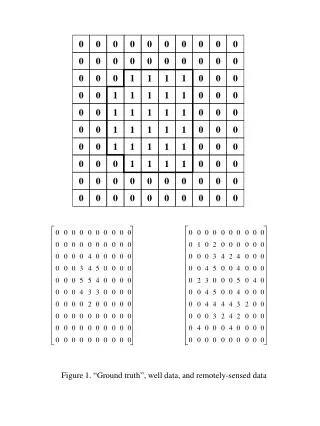
0 0 0 0 0 0 0 0 0 0 0 0 0 0 0 0 0 0 0 0 0 0 0 1 1 1 1 0 0 0 0 0 1 1 1 1 1 0 0 0 0 0 1 1 1 1 1 0 0 0 0 0 1 1 1 1 1 0 0 0 0 0 1 1 1 1 1 0 0 0 0 0 0 1 1 1 1 0 0 0 0 0 0 0 0 0 0 0 0 0 0 0 0 0 0 0 0 0 0 0 0 0 0 0 0 0 0 0 0 0 0 0 0 0 0 0 0 0 0 0 0 0 0 0 4 0 0 0 0 0 0 0 0 3 4 5 0 0 0 0 0 0 0 5 5 4 0 0 0 0 0 0 0 4 3 3 0 0 0 0 0 0 0 0 2 0 0 0 0 0 0 0 0 0 0 0 0 0 0 0 0 0 0 0 0 0 0 0 0 0 0 0 0 0 0 0 0 0 0 0 0 0 0 0 0 0 0 0 0 0 0 1 0 2 0 0 0 0 0 0 0 0 0 3 4 2 4 0 0 0 0 0 4 5 0 0 4 0 0 0 0 2 3 0 0 0 5 0 4 0 0 0 4 5 0 0 4 0 0 0 0 0 4 4 4 4 3 2 0 0 0 0 0 3 2 4 2 0 0 0 0 4 0 0 0 4 0 0 0 0 0 0 0 0 0 0 0 0 0 0 Figure 1. “Ground truth”, well data, and remotely-sensed data
255 Both brighter image and enhanced contrast Slope = Contrast of original image Dimmer (more contrast) Brighter (less contrast) 0 60 200 255 Figure 2. Several options in histogram equalization
1250.0 1000.0 800.0 630.0 500.0 400.0 315.0 250.0 200.0 150.0 125.0 100.0 80.0 63.0 50.0 40.0 31.5 100 95 90 85 80 75 70 100 95 90 85 80 75 70 100 95 90 85 80 75 70 100 95 90 85 80 75 70 100 95 90 85 80 75 70 100 95 90 85 80 75 70 100 95 90 85 80 75 70 100 95 90 85 80 75 70 100 95 90 85 80 75 70 100 95 90 85 80 75 70 100 95 90 85 80 75 70 100 95 90 85 80 75 70 100 95 90 85 80 75 70 100 95 90 85 80 75 70 100 95 90 85 80 75 70 100 95 90 85 80 75 70 100 95 90 85 80 75 70 Center Frequency - Hz Grey scale Levels - dB Figure 3. Grey scale definition (Banaszak et al. 1997)
@ t = 2.8 sec t = 0.5 sec Figure 4. Sound levels in decibels (Banaszak et al. 1997)
GOAL SOCIAL ENVIRONMENT ECONOMICS – Aesthetics – Property Values – Traffic Impacts – Land Use – Accessibility – Tip Fees – Tax Revenues – Out-of-District Revenues – Jobs – Noise and Odor – Ecology – Health Risks – Air – Ground Water Figure 5. Hierarchy of a Municipal Solid Waste Problem
Rate: 0.20 1 78 24 4 Rate: 0.10 50 100 5 Rate: 0.25 Rate: 0.35 3 32 102 16 Rate: Maintenance Call Arrival Rate Rate: 0.10 2 Figure 6. Service Network (Patterson 1995)
1 4 5 3 2 Figure 7. Multi-commodity Flow (Patterson 1995)
2 1 5 3 3 1 2 7 2 4 5 5 3 3 6 4 Legend __x__ (travel time) Figure 8. Travelling Salesman Problem
Legend x (travel time in State 1) x (travel time in State 2) (demand in State 1) (demand in State 2) 2 2´ 1 4 2 4.5 3.5 1.5 4 1 1 2.5 4 6 3´ 2 2 5.5 3 1 Figure 9. Stochastic Facility-Location and Routing
2 C32 = 50+x32 C24 = 10x24 x1 x3 C34 = 10+x34 4 5 x2 C14 = 50+x14 C13 = 10x13 1 Legend x Flow C Time Figure 10. Illustrating Braess’ Paradox.
HOTEL SEVEN HOTEL THREE HOTEL EIGHT HOTEL FOUR HOTEL TWO HOTEL FIVE HOTEL ONE HOTEL SIX 80 – 70 – 60 – 50 – 40 – 30 – 20 – 10 – 0 – -10 – -20 – -30 – 80 – 70 – 60 – 50 – 40 – 30 – 20 – 10 – 0 – -10 – -20 – -30 – 80 – 70 – 60 – 50 – 40 – 30 – 20 – 10 – 0 – -10 – -20 – -30 – 80 – 70 – 60 – 50 – 40 – 30 – 20 – 10 – 0 – -10 – -20 – -30 – 80 – 70 – 60 – 50 – 40 – 30 – 20 – 10 – 0 – -10 – -20 – -30 – 80 – 70 – 60 – 50 – 40 – 30 – 20 – 10 – 0 – -10 – -20 – -30 – 80 – 70 – 60 – 50 – 40 – 30 – 20 – 10 – 0 – -10 – -20 – -30 – 80 – 70 – 60 – 50 – 40 – 30 – 20 – 10 – 0 – -10 – -20 – -30 – PICKUP PICKUP PICKUP PICKUP PICKUP PICKUP PICKUP PICKUP | 0 | 0 | 0 | 0 | 0 | 0 | 0 | 0 | 50 | 50 | 50 | 50 | 50 | 50 | 50 | 50 | 100 | 100 | 100 | 100 | 100 | 100 | 100 | 100 | 150 | 150 | 150 | 150 | 150 | 150 | 150 | 150 | 200 | 200 | 200 | 200 | 200 | 200 | 200 | 200 | 250 | 250 | 250 | 250 | 250 | 250 | 250 | 250 | 300 | 300 | 300 | 300 | 300 | 300 | 300 | 300 | 350 | 350 | 350 | 350 | 350 | 350 | 350 | 350 | 400 | 400 | 400 | 400 | 400 | 400 | 400 | 400 DAY DAY DAY DAY DAY DAY DAY DAY Figure 11. Time sequence plots of pickup percentages (Pfeifer and Bodily 1990)
50– 40 – 30 – 20 – 10 – 0 – 49.2 38.1 37.3 33.85 32.4 29.9 Arsenic g/l 25.6 25.4 18.4 18.3 17.1 16.2 17.3 16 15.5 13.9 11.6 15.1 12.1 11.8 10 10 10 10 10 10 10 10 10 10 10 10 10 10 10 10 10 10 10 2.7 2.9 0 5 10 15 20 25 30 35 40 Time t in weeks 50– 40 – 30 – 20 – 10 – 0 – 42.9 37.15 35 28 28.6 Arsenic g/l 22.44 22.3 19.85 18 16.65 21.25 15.7 17 15.5 14.6 13.6 14.8 11.2 12.6 10.8 10 10 10 10 10 10 10 10 10 10 10 10 10 10 10 10 10 10 10 10 3.1 0 5 10 15 20 25 30 35 40 Time t in weeks 80– 64 – 48 – 32 – 16 – 0 – 40.3 Arsenic g/l 24.5 26.5 20.1 22.6 22.2 19.7 14.4 13.4 15 13.2 12.8 11.7 11.4 13.7 14.2 10.5 12.8 12.34 12.4 11.4 10.725 10 10 10 10 10 10 10 10 10 10 10 10 10 10 10 10 10 10.325 6.5 0 5 10 15 20 25 30 35 40 Time t in weeks Figure 12. Contamination time-series for wells 1,2 and 3 (Wright 1995)