Spatial Processes and Land-atmosphere Flux
670 likes | 853 Vues
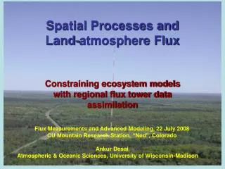
Spatial Processes and Land-atmosphere Flux. Constraining ecosystem models with regional flux tower data assimilation. Flux Measurements and Advanced Modeling, 22 July 2008 CU Mountain Research Station, “Ned”, Colorado Ankur Desai Atmospheric & Oceanic Sciences, University of Wisconsin-Madison.

Spatial Processes and Land-atmosphere Flux
E N D
Presentation Transcript
Spatial Processes andLand-atmosphere Flux Constraining ecosystem models with regional flux tower data assimilation Flux Measurements and Advanced Modeling, 22 July 2008 CU Mountain Research Station, “Ned”, Colorado Ankur Desai Atmospheric & Oceanic Sciences, University of Wisconsin-Madison
Why regional? • Spatial interpolation/extrapolation • Evaluation across scales • Landscape level controls on biogeochem. • Understand cause of spatial variability • Emergent properties of landscapes
Why regional? Courtesy: Nic Saliendra
Why regional? • NEP (=-NEE) at 13 sites • Stand age matters • Ecosystem type matters • Is interannual variability coherent? • Are we sampling sufficient land cover types”?
Why data assimilation? • Meteorological, ecosystem, and parameter variability hard to observe/model • Data assimilation can help isolate model mechanisms responsible for spatial variability • Optimization across multiple types of data • Optimization across space
Why data assimilation? • Old way: • Make a model • Guess some parameters • Compare to data • Publish the best comparisons • Attribute discrepancies to error • Be happy
Why data assimilation? • New way: • Constrain model(s) with observations • Find where model or parameters cannot explain observations • Learn something about fundamental interactions • Publish the discrepancies and knowledge gained • Work harder, be slightly less happy, but generate more knowledge
Back to those stats… [A|B] = [AB] / [B] [P|D] = ( [D|P] [P] ) / [D] (parameters given data) = [ (data given parameters)× (parameters) ] / (data) Posterior = (Likelihood x Prior) / Normalizing Constraint
For the visually minded • D Nychka, NCAR
Some case studies • Prediction • Up and down scaling • Regional evaluation • Interannual variability • Forest disturbance and succession
Sipnet • A “simplified” model of ecosystem carbon / water and land-atmosphere interaction • Minimal number of parameters • Driven by meteorological forcing • Still has >60 parameters • Braswell et al., 2005, GCB • Sacks et al., 2006, GCB added snow • Zobitz et al., 2008
Parameter estimation • MCMC is an optimizing method to minimize model-data mismatch • Quasi-random walk through parameter space (Metropolis) • Prior parameters distribution needed • Start at many random places (Chains) in prior parameter space • Move “downhill” to minima in model-data RMS by randomly changing a parameter from current value to a nearby value • Avoid local minima by occasionally performing “uphill” moves in proportion to maximum likelihood of accepted point • Use simulated annealing to tune parameter space exploration • Pick best chain and continue space exploration • Requires ~500,000 model iterations (chain exploration, spin-up, sampling) • End result – “best” parameter set and confidence intervals (from all the iterations) • NEE, Latent Heat Flux (LE), Sensible Heat Flux (H), soil moisture can all be used • Nighttime NEE good measure of respiration, maybe H? • Daytime NEE, LE good measures of photosynthesis • SipNET is fast (<10 ms year-1), so good for MCMC (4 hours for 7yr WLEF) • Based on PNET ecosystem model • Driven by climate, parameters and initial carbon pools • Trivially parallelizable (needs to be done, though)
2 years = 7 years 1997 1998 1999 2000 2001 2002 2003 2004 2005
Simple comparisons… Desai et al, 2008, Ag For Met
We need to do better • Lots of flux towers (how many?) • Lots of cover types • A very simple model • Have to think about the tall tower flux, too • What does it sample?
Multi-tower synthesis aggregation with large number of towers (12) in same climate space • towers mapped to cover/age types • parameter optimization with minimal 2 equation model
Tall tower downscaling • Wang et al., 2006
Scaling evaluation • Desai et al., 2008
Now we can wildly extrapolate • Take 17 towers • Fill the met data • Use a simple model to estimate parameters for each tower using MCMC • Apply parameters to other region meteorology data • Scale to region by cover/age class
Another simple(r) model • No carbon pools • GPP model driven by LAI, PAR, Air temp, VPD, Precip • LAI model driven by GDD (leaf on) and soil temp (leaf off) • 3 pool ER, driven by Soil temp and GPP • 19 parameters, fix 3
20 yr regional NEE • Cover types + • Age structure + • Parameters • Forcing for a lake organic carbon input model
IAV • Does growing season start explain IAV? • Can a very simple model be constructed to explain IAV? • Hypothesis: growing season length explains IAV • Can we make a cost function more attuned to IAV? • Hypothesis: MCMC overfits to hourly data
New cost function • Original log likelihood computes sum of squared difference at hourly • What if we also added monthly and annual squared differences to this likelihood? • Have to scale these less frequent values