Spatial processes and statistical modelling
Spatial processes and statistical modelling. Peter Green University of Bristol, UK IMS/ISBA, San Juan, 24 July 2003. . . . . . . . . Spatial indexing. Continuous space Discrete space lattice irregular - general graphs areally aggregated Point processes

Spatial processes and statistical modelling
E N D
Presentation Transcript
Spatial processes and statistical modelling Peter Green University of Bristol, UK IMS/ISBA, San Juan, 24 July 2003
Spatial indexing • Continuous space • Discrete space • lattice • irregular - general graphs • areally aggregated • Point processes • other object processes
Purpose of overview • setting the scene for 8 invited talks on spatial statistics • particularly for specialists in the other 2 areas
Perspective of overview • someone interested in the development of methodology • for the analysis of spatially-indexed data • probably Bayesian • models and frameworks, not applications • personal, selective, eclectic
Genesis of spatial statistics • adaptation of time series ideas • ‘applied probability’ modelling • geostatistics • application-led
Space vs. time • apparently slight difference • profound implications for mathematical formulation and computational tractability
Requirements of particular application domains • agriculture (design) • ecology (sparse point pattern, poor data?) • environmetrics (space/time) • climatology (huge physical models) • epidemiology (multiple indexing) • image analysis (huge size)
Key themes • conditional independence • graphical/hierarchical modelling • aggregation • analysing dependence between differently indexed data • opportunities and obstacles • literal credibility of models • Bayes/non-Bayes distinction blurred
A big subject…. Noel Cressie: “This may be the last time spatial statistics is squeezed between two covers” (Preface to Statistics for Spatial Data, 900pp., Wiley, 1991)
Why build spatial dependence into a model? • No more reason to suppose independence in spatially-indexed data than in a time-series • However, substantive basis for form of spatial dependent sometimes slight - very often space is a surrogate for missing covariates that are correlated with location
Modelling spatial dependence in discretely-indexed fields • Direct • Indirect • Hidden Markov models • Hierarchical models
Hierarchical models, using DAGs Variables at several levels - allows modelling of complex systems, borrowing strength, etc.
Modelling with undirected graphs Directed acyclic graphs are a natural representation of the way we usually specify a statistical model - directionally: • disease symptom • past future • parameters data …… whether or not causality is understood. But sometimes (e.g. spatial models) there is no natural direction
X0 X1 X2 X3 X4 Conditional independence In model specification, spatial context often rules out directional dependence (that would have been acceptable in time series context)
Conditional independence In model specification, spatial context often rules out directional dependence X20 X21 X22 X23 X24 X10 X11 X12 X13 X14 X00 X01 X02 X03 X04
Conditional independence In model specification, spatial context often rules out directional dependence X20 X21 X22 X23 X24 X10 X11 X12 X13 X14 X00 X01 X02 X03 X04
a b Directed acyclic graph c in general: d for example: p(a,b,c,d)=p(a)p(b)p(c|a,b)p(d|c) In the RHS, any distributions are legal, and uniquely define joint distribution
Undirected (CI) graph Regular lattice, irregular graph, areal data... X20 X21 X22 Absence of edge denotes conditional independence given all other variables X10 X11 X12 X00 X01 X02 But now there are non-trivial constraints on conditional distributions
Undirected (CI) graph () X20 X21 X22 clique X10 X11 X12 X00 X01 X02 The Hammersley-Clifford theorem says essentially that the converse is also true - the only sure way to get a valid joint distribution is to use ()
Hammersley-Clifford A positive distribution p(X) is a Markov random field X20 X21 X22 X10 X11 X12 if and only if it is a Gibbs distribution X00 X01 X02 - Sum over cliques C (complete subgraphs)
Partition function Almost always, the constant of proportionality in X20 X21 X22 X10 X11 X12 is not available in tractable form: an obstacle to likelihood or Bayesian inference about parameters in the potential functions Physicists call the partition function X00 X01 X02
where Gaussian Markov random fields: spatial autoregression If VC(XC)is -ij(xi-xj)2/2for C={i,j}and 0 otherwise, then is a multivariate Gaussian distribution, and is the univariate Gaussian distribution
non-zero non-zero A B C D Gaussian random fields A B C D Inverse of (co)variance matrix: dependent case A B C D
Gaussian Markov random fields: spatial autoregression Distinguish these conditional autoregression (CAR) models from the corresponding simultaneous autoregression (SAR) models i.i.d. normal (cf time series case). The latter are less compatible with hierarchical model structures.
Non-Gaussian Markov random fields Pairwise interaction random fields with less smooth realisations obtained by replacing squared differences by a term with smaller tails, e.g.
Agricultural field trials • strong cultural constraints • design, randomisation, cultivation effects • 1-D analysis in 2-d fields • relationships between IB designs, splines, covariance models, spatial autoregression…
Discrete Markov random fields Besag (1974) introduced various cases of for discrete variables, e.g. auto-logistic (binary variables), auto-Poisson (local conditionals are Poisson), auto-binomial, etc.
is Bernoulli(pi) with Auto-logistic model (Xi= 0 or 1) - a very useful model for dependent binary variables (NB various parameterisations)
Statistical mechanics models The classic Ising model (for ferromagnetism) is the symmetric autologistic model on a square lattice in 2-D or 3-D. The Potts model is the generalisation to more than 2 ‘colours’ and of course you can usefully un-symmetrise this.
is Poisson Auto-Poisson model For integrability, ij must be 0, so this only models negative dependence: very limited use.
Hierarchical models and hidden Markov processes
Chain graphs • If both directed and undirected edges, but no directed loops: • can rearrange to form global DAG with undirected edges within blocks
Chain graphs • If both directed and undirected edges, but no directed loops: • can rearrange to form global DAG with undirected edges within blocks • Hammersley-Clifford within blocks
Hidden Markov random fields • We have a lot of freedom modelling spatially-dependent continuously-distributed random fields on regular or irregular graphs • But very little freedom with discretely distributed variables • use hidden random fields, continuous or discrete • compatible with introducing covariates, etc.
Hidden Markov models e.g. Hidden Markov chain z0 z1 z2 z3 z4 hidden y1 y2 y3 y4 observed
Hidden Markov random fields Unobserved dependent field Observed conditionally-independent discrete field (a chain graph)
relative risk Spatial epidemiology applications expected cases independently, for each region i. Options: • CAR, CAR+white noise (BYM, 1989) • Direct modelling of ,e.g. SAR • Mixture/allocation/partition models: • Covariates, e.g.: cases
Spatial epidemiology applications Spatial contiguity is usually somewhat idealised
CAR model for lip cancer data (WinBUGS example) random spatial effects regression coefficient covariate expected counts observed counts
Example of an allocation model Richardson & Green (JASA, 2002) used a hidden Markov random field model for disease mapping observed incidence relative risk parameters expected incidence hidden MRF
z k e Y Chain graph for disease mapping based on Potts model
Larynx cancer in females in France SMRs
Continuously indexed fields The basic model is the Gaussian random field with and Translation-invariant or fully stationary (isotropic) cases have and or ,resp.
Geostatistics and kriging • There is a huge literature on a group of methodologies originally developed for geographical and geological data • The main theme is prediction of (functionals of) a random field based on observations at a finite set of locations
Ordinary kriging • is a random process, we have observations and we wish to predict , e.g. a “block average” • The usual basis is least-squares prediction, using a model for the mean and covariance of estimated from the data
Ordinary kriging The usual assumption is that is intrinsically stationary, i.e. has 2nd order structure for all s is called the semi-variogram This is somewhat weaker than full 2nd-order stationarity
Ordinary kriging The optimal solution to the prediction problem in terms of the semivariogram follows from standard linear algebra arguments; an empirical estimate of the semivariogram is then plugged in.
Variants of kriging Kriging without intrinsic stationarity (& a model instead of empirical estimates) Co-kriging (multivariate) Robust kriging Universal kriging (kriging with regression) Disjunctive (nonlinear) kriging Indicator kriging Connections with splines