Introduction to Spatial modelling
Introduction to Spatial modelling. Duncan Lee and Marian Scott March / April 2009. Statistics for Environmental Evaluation. Outline. Geostatistics Areal unit data Spatial point processes Spatio-temporal modelling. 1. Geostatistical data.

Introduction to Spatial modelling
E N D
Presentation Transcript
Introduction to Spatial modelling Duncan Lee and Marian Scott March / April 2009 Statistics for Environmental Evaluation
Outline • Geostatistics • Areal unit data • Spatial point processes • Spatio-temporal modelling
1. Geostatistical data • For a fixed region A, the variable of interest could be measured at any location. • However due to time/cost constraints it has only been measured at n locations u1,…, un , which are typically chosen and not random. • The random variables measured at all n locations are denoted by Z(u1),…, Z(un) . • Examples of geostatistical data include air pollution, temperature, water quality.
Example – Air pollution Location of the pollution monitors in Greater London.
Goals of geostatistics • Given observations Z(u1),…, Z(un), there are two stages in a general geostatistical analysis. • How do I best to model the data? • How do I use my model to estimate quantities of interest? For example: • How do I estimate Z(u0) where u0 is an unobserved location? • How do I draw a map of Z(u) for all points u in my region? • How do I estimate the average value over the region?
Modelling geostatistical data • When modelling geostatistical data we need to consider the following: • Are the observations Z(u1),….Z(un) Gaussian or do I need to transform them? • Is there a pronounced spatial trend that needs to be modelled – e.g. regression variables or other trends. • Are the responses spatially dependent – i.e. how are observations close to each other in space related? • Which method of analysis should I use – e.g. frequentist or Bayesian methods?
A general model for data Z=(Z(u1),…, Z(un)), is Z = µ + S Where The data Z are assumed to be normally distributed. µ is the mean function and models spatial trend. S is a stochastic process and models spatial dependence. General geostatistical model
Modelling the spatial trend µ • A spatial trend is a systematic change in the mean function µ over the area of interest. It is generally smooth, although it may change abruptly in response to environmental forcing variables (e.g., bedrock geology, presence of mountains, etc). It can be modelled in numerous ways. • Regression variables such as geology or altitude. • Polynomials or smooth functions in the co-ordinates u1…un. • Modelled within the spatial dependence component S, although we wont discuss this here.
Types of spatial dependence 1 • Spatial dependence quantifies how the values of Z(u1),…, Z(un) are related to each other. Three types of spatial dependence are possible. • Independence - the values of Z(u1),…, Z(un) are not related. • Negative dependence – if locations u1 and u2 are close together then Z(u1) and Z(U2) will have different values. • Positive dependence – if locations u1 and u2 are close together then Z(u1) and Z(U2) will have similar values.
Types of spatial dependence 2 • There are two common simplifying assumptions that are made when modelling spaital dependence in Geostatistical data. • Stationarity – Spatial dependence is stationary over a region R if the dependence between [Z(u0),Z(U1)] is the same as the dependence between [Z(u0+m), Z(U1+m)] for any location shift m. • Isotropy – Spatial dependence is isotropic if the dependence between observations at two locations a distance d apart, is the same no matter what direction you have to travel to get from the first to the second location.
Common spatial dependence • The most common type of spatial dependence is positive, i.e. the closer two locations are the more similar their values will be. Therefore, for the remainder of this course we: • assume positive spatial dependence rather than negative. • assume that any spatial trend has been removed by the mean function µ. • assume that the spatial dependence is stationary and isotropic.
Modelling spatial dependence • A common model for spatial dependence is given by • S ~ N(0 , V) • which implies the data are normally distributed. • Here V is the variance-covariance matrix, and is a transformed correlation matrix. If all observations have the same variance, then we can write • V=σ2C • C is the correlation matrix. • σ2 is the common variance of each observation.
Structure of the correlation matrix 1 • The correlation matrix C typically has the following characteristics. • The diagonal elements equal 1, as they represent the correlation of an observation with itself. • The ijth element of C is close to one if locations ui and uj are close. • As locations ui and uj get further apart, the ijth element gets closer to zero. • Negative dependence (i.e. negative values in C) is rarely seen in geostatistical data.
Structure of the correlation matrix 2 • As we focus only on stationary and isotropic spatial dependence in this course, it means that: • The correlation between observations at two locations only depends on their distance and direction from each other not the actual locations (stationarity). • The correlation between observations at two locations only depends on their distance apart and not the direction between them (Isotropy).
Assuming the spatial dependence is stationary and isotropic, the covariance function between 2 points Z(u) and Z(u + t) simplifies to • a function of the scalar distance, t, between the two points. Similarly the correlation function is given by • Where σ2 is the variance and also denoted by V(0).
Semi-variogram modelling • However in the geostatistical literature spatial dependence is typically modelled in terms of a transformation of the variance or correlation function V(t) or C(t). This function is given by • γ(t) = 0.5Var(Z(u+t) – Z(u)) • = C(0) – C(t) • = σ2 - C(t) • and is called the semi-variogram.
Estimating the semi-variogram • The semi-variogram is given by γ(t) = σ2 - C(t), and is a function of the distance between two points t. There are two general approaches to estimating it. • Estimate and plot (t, γ(t)) from observations at all pairs of locations. • For each value t, estimate the average value γ(t) from all sets of observations that have locations a distance t apart.
Semi-variogram cloud The first option is the semi-variogram cloud, which for all pairs of points is a plot of against This form gives more than one value γ(t) for each value t, and so gives a scatterplot. Note the formula for semi-variogram again is γ(t) = 0.5Var(Z(u+t) – Z(u)) = σ2 - C(t)
Semi-variogram estimator The semi-variogram for data Z(u1),…, Z(un) can be estimated by calculating for any value of t. Here N(t) is the set of points (ui, uj) that are distance t apart. This function is called the empirical semi-variogram, and it can be plotted against t to see the general shape.
But what should γ(t) look like? γ(t) = σ2 - C(t)
The nugget is the limiting value of the semi-variogram as the distance t approaches zero. It quantifies the amount of spatial variability at very small spatial scales (those less than the separation between observations) and also measurement error. • The sill is the horizontal asymptote of the variogram, if it exists, and represents the overall variance of the random process, σ2. • The range is the distance t* at which the semi-variogram reaches the sill. Pairs of points that are further apart than the sill are uncorrelated
But what about in practice? • Sometimes the semi-variogram only approaches the sill asymptotically, and in this case we define the practical range as the lag t* at which • γ(t) = 0.95* sill • = 0.95* σ2
Examples in R • To see how the shape of the semi-variogram corresponds to the smoothness and variation in a spatial surface, we use the R package rpanel for illustration.
Semi-variogram models A number of semi-variogram models exist that can be used. Nugget - random data Spherical Exponential Although these models may not fit the data particularly well.
Modelling spatial dependence • This gives us a three stage process by which to model spatial data. • Determine the form of the mean function and subtract it from the observed data to form residuals. • Plot the empirical semi-variogram and determine which family of semi-variogram models it resembles. • Estimate the parameters of the mean function and the chosen semi-variogram model (sill, nugget, range) by least squares methods.
Goals of spatial prediction • Once a trend and spatial dependence model have been fitted, it is of interest to estimate the variable Z at some unobserved location u0. This could be because: • You want to know the value at an unobserved location of particular interest. • You want to draw a map of the levels of the variable across a region – e.g. a city or country. • You want to estimate the average level of a variable across a region.
Implementing spatial prediction • There are many methods for carrying out spatial prediction, including: • Regression modelling using generalised least squares. • Inverse distance weighted interpolation. • Kriging. • Bayesian spatial prediction • Most of these can be relatively easily implemented in modern statistical packages such as R.
Form of spatial prediction The majority of these approaches predict z*(u0) the variable at location u0 by a weighted average of the form The main difference between the methods is how the weights are estimated. A map can then be produced by predicting the surface at a regular grid of points.
Estimating a spatial average • Estimating the average value of a variable across a region (e.g. a electoral ward, city or country) can be done in numerous ways. One of the most straightforward is to extend single point prediction. • Predict the value of the variable at a set of locations P1,…..Pm that form a grid of equally spaced points across the region of interest. • Estimate the spatial average value as the average of these m prediction locations.
Example 137Cs deposition maps in SW Scotland prepared by different European teams (ECCOMAGS, 2002)
Ordinary Kriging • One popular method of spatial prediction is ordinary Kriging. It is implemented in a number of stages. • Estimate the spatial trend using least squares methods. • De-trend the observed values by subtracting off the trend, to obtain residuals that have no spatial trend. • Choose and fit a model for the variogram to the residuals, which produces the weights for the prediction . The idea behind kriging is to predict Z*(u0) from its conditional distribution given the observed data Z(u1),…..,Z(un).
Extending Kriging • There are a number of other kriging methods, such as: • Universal Kriging • block kriging, • The accuracy of the predictions will be unknown, so we can use kriging to produce uncertainty maps. • Recent work has been to develop approaches to incorporate this prediction uncertainty in the variogram model.
Kriging in R • There are routines to do kriging in the R libraries:- • geoR • fields • gstat • sgeostat • spatstat • spatdat
Choosing the locations • Suppose you can choose the locations u1,….,un at which you measure the variable of interest Z. Where should you choose to measure? • The desired set of locations depends on the goal of the analysis. • Point prediction – Locate points on a regular grid so that all prediction locations will be highly correlated with a few observed data points. • Average estimation – If the aim is to estimate the average value of Z over the region A, then correlated points provides redundant information. Therefore you want the distance between pairs of points to be roughly the variogram range.
2. Areal unit data • Suppose the region of interest A is split up into n non-overlapping sub-regions A1,….,An. • The variable of interest is only available as an aggregated average or total for each sub-region Ai. The data are denoted Z1,….Zn. • The lack of geostatistical data may be due to confidentiality reasons (e.g. personal data) or that the exact locations are just not recorded (e.g. election voting).
Motivating example • Lip cancer rates for the 56 counties in Scotland. Two possible questions of interest: • Does any environmental variable affect the number of new cases? • Is there an outbreak of lip cancer cases in any part of Scotland? • Map taken from a paper by Wakefield from Biostatistics 2007, 158-183.
Modelling areal unit data • When modelling areal unit data Z1,….,Zn from sub-regions A1,…,An consider the following: • Response distribution – normal, Poisson, binomial, etc. • Regression variables – e.g. sunlight in the lip cancer example. • Spatial dependence – how to model the spatial dependence? • Method of analysis – frequentist or Bayesian methods.
Modelling spatial dependence • In common with geostatistical data, spatial dependence will typically be positive rather than negative, I.e. the closer two areas (Ai, Aj) are, the more similar their values (Zi, Zj) will be. • There are two common methods for modelling spatial dependence in areal unit data: • Use a geostatistical model, where the locations of the data are assumed to come from the centre of the areal unit. • Use a model that is based on the notion of neighbours.
Defining neighbours • A common method for modelling positive dependence is based on an n by n neighbourhood or weight matrix W. • It comprises 1’s and 0’s, where element ij is 1 if areas i and j are neighbours and 0 otherwise. • Possible neighbours rules include • Areas sharing a common border. • Areas less than a distance d apart. • Area i is one of the closest areas in terms of distance to area j. A border specification
Conditional autoregressive models • For simplicity, assume that z1,…zn are normally distributed and there are no covariates (these assumptions can be relaxed). Then a conditional autoregressive (CAR) model is given by • Where • Z-i is the vector including all the elements of Z except the ith. • is the mean of Z in neighbouring areas of area i. • ni is the number of neighbours that area i has.
3. Spatial point processes • In Geostatistical and areal unit data types, observations are made at fixed locations or sub-regions across a region A. • For spatial point process data, it is the locations of the observations within the region A that are random and comprise the data. • Additional data may be collected at each location (marked point process). • Examples include lightning strikes and the locations of trees in a forest. • A realisation from a spatial point process is termed a spatial point pattern – a countable collection of events at locations u1,…un.
Notation • A spatial point process is defined for a region A. • Sub-regions within A are denoted A1, A2,…… • Single locations within A are denoted u1,u2,…… • Let N(A) be the random variable representing the number of events in the region A. • Similar defnitions apply to N(Ak) and N(uk).
Question of interest • The key question of interest for spatial point process data is • “Does the point pattern have any spatial dependence?” • Three general types of structure are possible. • Complete spatial randomness (CSR) – events occur at random. • Clustered process – events occur close to existing events. • Regular process – events occur away from existing events.
Example 1 Location of 65 Japanese black pine saplings in a square region of 5.7 metres squared.
Example 2 The locations of the centres of 42 biological cells observed under an optical microscope
How do you tell? So, having seen two examples of point processes, it’s not easy to determine whether a process is completely spatially random, clustered or regular. So how do you tell? The general idea is to Develop a statistical model for complete spatial randomness and see if the point process seem likely under that model. If they are then complete spatial randomness can be assumed. If not then we determine whether the point process looks more clustered or regular (the two opposite ends) than complete spatial randomness.
A model for CSR • Complete Spatial Randomness (CSR) asserts that: • (i) For any subregion Ak, N(Ak)~Poisson(|Ak|). • (ii) For disjoint sub-regions (A1, A2) , N(A1) and N(A2) are independent. • is termed the intensity and is the expected number of events per unit of area, so that |A| is the expected number of events in A. • A process satisfying (i) and (ii) is called a homogeneous Poisson process (with intensity ).
Mean and covariance • For a CSR process N(A)~Poisson(|A|). • Mean – The mean number of occurrences of a process is constant across the region A. Therefore at a single location u1, with unit area 1, the mean of N(u1) equals . • Variance – The variance of the number of occurrences equals the mean number of occurrences as a Poisson distribution is assumed. • Covariance – The spatial dependence of the process between two points (u1, u2) is determined by the second order intensity function 2 (u1, u2) . • However the latter is hard to work with.
The K function • Instead of working with the second order intensity function • 2 (u1, u2) to measure spatial dependence, we work with the • K function • K(t) = E{N0(t)} / • where N0(t) is the number of events within a distance t of an arbitrary event. So for a fixed • for large t, K(t) will be large • for small t, K(t) will be small t
Why is the K function useful? • Recall that • K(t) = E(n0 of events within t of an arbitrary event) / • For a CSR process - K(t) = t2 / = t2 - the area of a circle • For a clustered process we would expect more points close together than under CSR, so for small t, K(t) > t2. • For a regular process we would expect less points close together than under CSR, so for small t, K(t) < t2.