Ch 3.6: Variation of Parameters

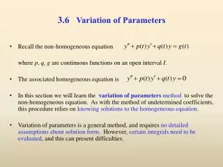
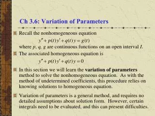
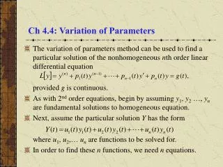
1. Ch 3.6: Variation of Parameters • Recall thenonhomogeneous equation where p, q,g are continuous functions on an open interval I. • The associated homogeneous equation is • In this section we will learn the variation of parameters method to solve the nonhomogeneous equation. As with the method of undetermined coefficients, this procedure relies on knowing solutions to homogeneous equation. • Variation of parameters is a general method, and requires no detailed assumptions about solution form. However, certain integrals need to be evaluated, and this can present difficulties.

2. Example: Variation of Parameters (1 of 6) • We seek a particular solution to the equation below. • We cannot use method of undetermined coefficients since g(t) is a quotient of sint or cost, instead of a sum or product. • Recall that the solution to the homogeneous equation is • To find a particular solution to the nonhomogeneous equation, we begin with the form • Then • or

3. Example: Derivatives, 2nd Equation (2 of 6) • From the previous slide, • Note that we need two equations to solve for u1 and u2. The first equation is the differential equation. To get a second equation, we will require • Then • Next,

4. Example: Two Equations (3 of 6) • Recall that our differential equation is • Substituting y'' and y into this equation, we obtain • This equation simplifies to • Thus, to solve for u1 and u2, we have the two equations:

5. Example: Solve for u1'(4 of 6) • To find u1 and u2 , we need to solve the equations • From second equation, • Substituting this into the first equation,

6. Example : Solve for u1 and u2(5 of 6) • From the previous slide, • Then • Thus

7. Example: General Solution (6 of 6) • Recall our equation and homogeneous solution yC: • Using the expressions for u1 and u2 on the previous slide, the general solution to the differential equation is

8. Summary • Suppose y1, y2 are fundamental solutions to the homogeneous equation associated with the nonhomogeneous equation above, where we note that the coefficient on y'' is 1. • To find u1 and u2, we need to solve the equations • Doing so, and using the Wronskian, we obtain • Thus

9. Theorem 3.7.1 • Consider the equations • If the functions p, q and g are continuous on an open interval I, and if y1 and y2 are fundamental solutions to Eq. (2), then a particular solution of Eq. (1) is and the general solution is