Sparse Bayesian Variable Selection in Medical Classification
In medical classification problems, selecting the right variables can impact data acquisition costs, classifier accuracy, and complexity. This study explores Tipping's sparse Bayesian learning method for variable selection, integrating it into various linear probablistic classifiers. Results show improved performance in cancer subtypes and disease classification. The methodology addresses uncertainties and algorithm sensitivities, enhancing model generalization and efficiency. This research provides insights for future experiments combining variable selection techniques.

Sparse Bayesian Variable Selection in Medical Classification
E N D
Presentation Transcript
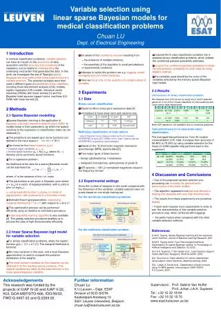
cancer no. samples no. genes task leukemia 72 7192 2 subtypes colon 62 2000 disease/normal Variable selection using linear sparse Bayesian models for medical classification problemsChuan LUDept. of Electrical Engineering 1 Introduction In medical classification problems, variable selectioncan have an impact on the economicsof data acquisition and the accuracy and complexityof the classifiers, and is helpful in understanding the underlying mechanism that generated the data. In this work, we investigate the use of Tipping’s sparse Bayesian learning method with linear basis functions in variable selection. The selected variables were then used in different types of probabilistic linear classifiers, including linear discriminant analysis (LDA) models, logistic regression (LR) models, relevance vector machines (RVMs) with linear kernels [1] and the Bayesian least squares support vector machines (LS-SVM) with linear kernels [3]. • reduced the 4-class classification problem into 6 pairwise binary classification problems, which yielded the conditional pairwise probability estimates. • coupled the conditional pairwise probability to obtain the joint posterior probability for each class by using Hastie’s method. • the variables used should be the union of the variables selected by the 6 binary sparse Bayesian logit models. • Be aware of the uncertainty involvedresulting from • – the existence of multiple solutions, • – the sensitivity of the algorithm to small perturbations of experimental conditions. • Attempts to tackle this problem are e.g. bagging, model averaging and committee machines. • Here we focus only on the selection of a single subset of variables. • 3.3 Results • LOO accuracy for binary classification problems. • We obtained zero LOO errors by using only 4 and 5 selected genes on 3 out of the 4 linear classifiers, for the Leukemia and colon cancer data respectively. • Note:’N/A’ stands for ’not available’ due to numerical problems. • Test performance for 4-class brain tumor classification. • The averaged test performance, from 30 random crossvalidation (CV) trials, increases from accuracy of 68.48% to 75.34% by using variable selection for the linear LS-SVM classifier that performs best in this experiment. • 4 Discussion and Conclusions • Use of the proposed variable selection pre-processing can increase the generalization performance of the linear models. • The algorithm appeared to be fast and efficient in dealing with datasets with very high dimentionality. • The results from these experiments are somehow biased • Future work requires more experiments in order to see the characteristics of this variable selection procedure (esp. when combined with bagging) • the performance when compared with the other variable selection methods. • References • [1] M.E. Tipping, Sparse Bayesian learning and the relevance vector machine. Journal of Machine Learning Research, 2001. • [2] M.E. Tipping and A. Faul, Fast marginal likelihood maximisation for sparse Bayesian models. In Proceedings of Artificial Intelligence and Statistics ’03, 2003. • [3] J.A.K. Suykens, T. Van Gestel et al., Least Squares Support Vector Machines. Singapore: World Scientific, 2002. • [4] I. Guyon et al., Gene selection for cancer classification using support vector machines, Machine learning, 2002. • [5] L. Lukas, A. Devos et al., Classification of brain tumours using 1H MRS spectra, internal report, ESAT-SISTA, K.U.Leuven, 2003. • 3 Experiments • 3.1 Data • Binary cancer classification • Based on Micro-array gene expression data [4] • normalized to have mean zero and variance one. • Multiclass classification of brain tumors • * Use of the brain tumor data provided by the EU funded INTERPRET project (IST-19999-10310, http:// carbon.uab.es/ INTERPRET) is gratefully acknowledged • Based on the 1H short echo magnetic resonance spectroscopy (MRS) spectra data [5]. • Four major types of brain tumors: • – benign (glioblastomas, metastases) • – malignant (menigiomas, astrocytomas of grade II). • 205 spectra 138 L2 normalized magnitude values in the frequency domain • 3.2 Experimental settings • Since the number of samples is very small compared with the dimension of the variables, variable selection was not purely based on one single training set. • For the two binary classification problems • For the multiclass classification problem • 2 Methods • 2.1 Sparse Bayesian modelling • Sparse Bayesian learning is the application of Bayesian automatic relevance determination (ARD)to models linear in their parameters, by which the sparse solutions to the regression or classification tasks can be obtained [1]. • The predictions are based upon some functions y(x) defined in the input space x: • Two forms for the basis functions m(x): • – Original input variablesm= xm • – Kernel basis functionm= K(x; xm), where K(:; :) denotes some symmetric kernel functions. • For a regression problem, • the likelihood of the data for a sparse Bayesian model can be expressed as: • where 2 is the variance of the i.i.d. noise. • The parameters w are given a Gaussian prior where = {m} is a vector of hyperparameters, with a uniform prior on log(m). • using a penalty function mlog|wm| in terms of regularization, with preference to a smoother model. • Estimate these hyperparameters: maximizing marginal likelihood p(T | w; 2)with respect to and 2. • This optimization process can be performed efficiently using an iterative re-estimation procedure. • A fast sequential learning algorithmis also available [2]. The greedy selection procedure enables us to process the data of high dimensionality efficiently. • 2.2 linear Sparse Bayesian logit model for variable selection • For binary classification problems, utilize the logistic function g(y) = 1/(1 + e-y) [1]. The marginal likelihood is binomial. • No noise variance in this case, and a local Gaussian approximation is used to compute the posterior distribution of the weights. • The most relevant variables for this classifier can be obtained from the resulting sparse solutions, if the original variables are taken as the basis function in the linear sparse Bayesian classifier. Acknowledgements This research was funded by the projects of IUAP IV-02 and IUAP V-22, KUL GOA-MEFISTO-666, IDO/99/03, FWO G.0407.02 and G.0269.02. Further information Chuan Lu K.U.Leuven – Dept. ESAT Division of SCD-SISTA Kasteelpark Arenberg 10 3001 Leuven (Heverlee), Belgium chuan.lu@esat.kuleuven.ac.be Supervisors: Prof. Sabine Van Huffel Prof. Johan J.A.K. Suykens Tel.: +32 16 32 18 84 Fax: +32 16 32 19 70 www.esat.kuleuven.ac.be