Download
1 / 35
350 likes | 1.16k Vues
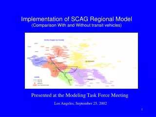
Implementation of SCAG Regional Model (Comparison With and Without transit vehicles). Presented at the Modeling Task Force Meeting. Los Angeles, September 25, 2002. Comparison of Multi-class Assignment with and without Transit Vehicles (Base year 1997, AM period).

E N D
Implementation of SCAG Regional Model(Comparison With and Without transit vehicles) Presented at the Modeling Task Force Meeting Los Angeles, September 25, 2002
Comparison of Multi-class Assignment with and without Transit Vehicles (Base year 1997, AM period) • Given data (base year 1997, AM period): • highway and transit route network in TRANPLAN format; • Mode Choice output trip tables • 6 trip tables from TRANPLAN model run; • drive alone, car pool 2, and car pool 3+; • light, medium and heavy heavy duty trucks; • EMME2 converted the TRANPLAN files automatically; • Transit vehicles equivalent factor = 2.5 autos; • Run EMME/2 auto-truck multi-class assignment macro developed for the SCAG Regional Model, with and without transit vehicles; • Compare link volume of the two runs;
EMME/2 Databank for the SCAG Regional Model • Zone: 3325 • 3217 ;SCAG region zone and externals • 108 ;zones converted from parking lots • Regular nodes: 26290 • Directional links: 108897 • Transit lines: 672 • Transit line segments: 60926
Trip Tables for the Highway Assignment • Total trips: - drive alone: 5319853 - light heavy duty trucks: 85040 - car pool 2: 1625165 - medium heavy duty trucks: 62804 - car pool 3+: 430209 - heavy heavy duty trucks: 38333
EMME/2 Auto-Truck Assignment Convergence Measures • Relative difference (R.D.) at iteration l between the flow calculated based on the shortest path problem with a network loading of flow and the last flow: SUM( ABS (flow difference between iteration l and l-1) ) R.D. = * 100 SUM (flow at iteration l ) • Relative gap (Rgap) at iteration l which measures the relative difference between the total travel cost and the travel cost on shortest paths at iteration l (Total travel cost - Travel cost on sh. path ) Rgap = * 100 Total travel cost where: travel cost = SUM (link travel time * link volume)
TRANPLAN Assignment Results with Iterations V E H I C L E C O S T - O F - T R A V E L S U M M A T I O N S S1= S2= ERROR= ITERATION V(LINK)*I(LINK) V(O-D)*I(O-D) (S1-S2)/S1 LAMBDA FRACTION --------- --------------- ------------- ---------- ------ -------- 0 -- 1057422. -- 1.00000 .18605 1 4324790. 1416242. .67253 .188 .04293 2 2949963. 1451959. .50780 .180 .05016 3 2324005. 1480157. .36310 .195 .06775 4 1994479. 1472321. .26180 .211 .09273 5 1791530. 1473923. .17728 .133 .06733 6 1706574. 1482930. .13105 .164 .09950 7 1645334. 1484676. .09764 .148 .10571 8 1606160. 1474137. .08220 .133 .10907 9 1576393. 1479840. .06125 .086 .07721 10 1558673. 1490711. .04360 .102 .10156 11 1548724. -- --
Transit Vehicles (summary) • Total number of links with transit services: 26,920 • Total link length (miles) with transit services: 8,554 • Total vehicle miles traveled (auto equivalence): 33,793,331 • Total transit vehicle miles: 1,351,732 • Total transit vehicle hours (auto equivalence): 183,271 • Total transit vehicle hours: 73,308
Transit Vehicle’s VHT and VMT (by area type) Transit service are dense in the Urban CBD area.
Transit Vehicle’s VHT and VMT (by facility type) Transit service are dense on Principal Arterial and Primary Arterial.
VMT and VHT without Considering Transit Vehicles (by area type)
Speed Changes when Considering Transit Vehicles (by area type) Average speed reduced in Core area (-7.22 m/h) and CBD area (-2.89 m/h) is significant.
Speed Changes when Considering Transit Vehicles (by facility type) Average speed change is less than 1 mile per hour for all facilities.
Speed Changes when Considering Transit Vehicles (on freeway)
Speed Changes when Considering Transit Vehicles (on principal arterial)
Speed Changes when Considering Transit Vehicles (on primary arterial)
Speed Changes when Considering Transit Vehicles (on principal and primary arterial)
Speed Changes when Considering Transit Vehicles (LA downtown)
VMT and VHT Total Changes when Considering Transit Vehicles (transit vehicle included, by area type)
VMT and VHT Total Changes when Considering Transit Vehicles (transit vehicle included, by facility type)
VMT and VHT Pure Changes when Considering Transit Vehicles (transit vehicle not included, by area type)* VMT in Urban CBD decreases due to transit services, which increase the congestion and the travel time * It is to show the pure changes of auto-truck VMT and VHT after considering the transit vehicles. This is the influence of transit vehicles on the auto-truck flow.
VMT and VHT Pure Changes when Considering Transit Vehicles (transit vehicle not included, by facility type)* VMT on Principal Arterial decreases due to transit services, which increase the congestion and the travel time. Auto volume shifts to other facilities. * It is to show the pure changes of auto-truck VMT and VHT after considering the transit vehicles. This is the influence of transit vehicles on the auto-truck flow.
Implementation Sample Plots with ENIF (auto-truck volume without transit vehicles at LA downtown )
Implementation Sample Plots with ENIF (auto-truck volume with transit vehicles at LA downtown )
Implementation Sample Plots with ENIF (auto-truck volume changes at LA downtown transit vehicle volume was not shown*) * It is to show the pure changes of auto-truck volume after considering the transit vehicles. This is the influence of transit vehicles on the auto-truck flow.
Implementation Sample Plots with ENIF (auto-truck speed at LA downtown)
Implementation Sample Plots with ENIF (auto-truck speed decreased at LA downtown)
Implementation Sample Plots with ENIF (park-and-ride auto volume near LA downtown) VMT for park-and-ride: 663322, about 1% of the total VHT for park-and-ride: 23132, about 1% of the total This part is not yet considered in the SCAG TRANPLAN model.
Conclusions • Transit vehicles have a significant impact on the assignment: flow, travel time, VMT and VHT; • Transit vehicles have most impact on the flow on the Principal Arterial links and in the Business District; • The total increase in the VMT of the region is about 2.14 %; • The total increase in the VHT of the region is about 6.52 %; • If the park-and-ride volume is considered, the total VMT and VHT increase by about another 1 % each.